Environmental Geophysics
Frequency Domain Electromagnetic Methods
Basic Concept
In the frequency domain method, the transmitter emits a sinusoidally varying current at a specific frequency. For example, at a frequency of 100 Hz, the magnetic field amplitude at the receiver will be that shown in the top part of figure 1. Because the mutual inductance between the transmitter and conductor is a complex quantity, the electromagnetic force induced in the conductor will be shifted in phase with respect to the primary field, similar to the illustration in the lower part of figure 1. At the receiver, the secondary field generated by the currents in the conductor will also be shifted in phase by the same amount. There are three methods of measuring and describing the secondary field.
Amplitude and Phase
The amplitude of the secondary field can be measured and is usually expressed as a percentage of the theoretical primary field at the receiver. Phase shift, the time delay in the received field by a fraction of the period, can also be measured and displayed.
In Phase and Out-of-Phase Components
The second method of presentation is to electronically separate the received field into two components, as shown in the lower part of figure 1.
The first component is in phase with the transmitted field whereas the second component is exactly 90° out-of-phase with the transmitted field. The in‑phase component is sometimes called the real component, and the out-of-phase component is sometimes called the"quadrature" or "imaginary" component. Both of the above measurements require some kind of phase link between transmitter and receiver to establish a time or phase reference. This is commonly done with a direct wire link, sometimes with a radio link, or through the use of highly accurate, synchronized crystal clocks in both transmitter and receiver.
The simpler frequency domain EM systems are tilt angle systems that have no reference link between the transmitter and receiver coils. The receiver simply measures the total field irrespective of phase, and the receiver coil is tilted to find the direction of maximum or minimum magnetic field strength. As shown conceptually in figure 2, at any point the secondary magnetic field may be in a direction different from the primary field. With tilt angle systems, therefore, the objective is to measure deviations from the normal in-field direction and to interpret these in terms of geological conductors.
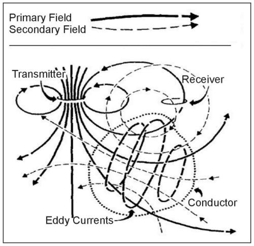
Figure 1. Generalized picture of electromagnetic induction prospecting. (Klein and Lajoie 1980; copyright permission granted by Northwest Mining Association and Klein)
The response parameter of a conductor is defined as the product of conductivity-thickness (σt), permeability (μ), angular frequency (ω = 2πf), and the square of some mean dimension of the target (a2). The response parameter is a dimensionless quantity. In MKS units, a poor conductor will have a response parameter of less than about 1, whereas an excellent conductor will have a response value greater than 1,000. The relative amplitudes of in-phase and quadrature components as a function of response parameter are given in figure 3 for the particular case of the sphere model in a uniform alternating magnetic field. For low values of the response parameter (< 1), the sphere will generally produce a low-amplitude out-of-phase anomaly; at moderate values of the response parameter (10-100), the response will be a moderate-amplitude in-phase and out-of-phase anomaly, whereas for high values of the response parameter (>1,000), the response will usually be in the in-phase component. Although figure 3 shows the response only for the particular case of a sphere in a uniform field, the response functions for other models are similar.
In frequency domain EM, depth and size of the conductor primarily affect the amplitude of the secondary field. The quality of the conductor (higher conductivity means higher quality) mainly affects the ratio of in-phase to out-of-phase amplitudes (AR/AI), a good conductor having a higher ratio (left side of figure 3) and a poorer conductor having a lower ratio (right side of figure 3).
Of the large number of electrical methods, many of them are in the frequency domain electromagnetic (FDEM) category and are not often used in geotechnical and environmental problems. Most used for these problems are the so-called terrain conductivity methods, VLF (very low frequency EM method), and a case of instruments called metal detectors.
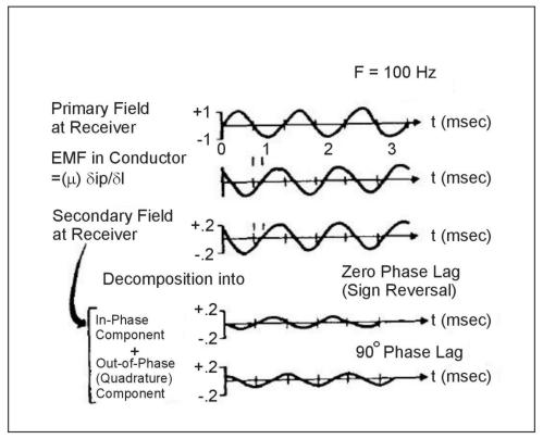
Figure 2. Generalized picture of the frequency domain EM method. (Klein and Lajoie 1980; copyright permission granted by Northwest Mining Association and Klein)
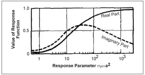
Figure 3. In-phase and out-of-phase response of a sphere in a uniform alternating magnetic field. (Klein and Lajoie 1980; copyright permission granted by Northwest Mining Association and Klein)
Data Interpretation
Interpretation of electromagnetic surveys follows basic steps. Most of the common EM systems have nomograms associated with them. Nomograms are diagrams on which the measured parameters, e.g., in-phase and out-of-phase components, are plotted for varying model conductivity and one or more geometrical factors, e.g., depth to top, thickness, etc. The model responses available for most electromagnetic methods are those of the long, thin dike (to model thin tabular bodies), a homogeneous earth, and a horizontal layer for simulating conductive overburden.
The first step is to attempt to determine from the shape of the anomaly a simple model geometry that can be thought to approximate the cause of the anomaly. The second step is to measure characteristics of the anomaly such as in-phase and out-of-phase amplitudes, and to plot these at the scale of the appropriate nomograms. From the nomogram and the shape of the anomaly, estimates generally can be made for quality of the conductor, depth to top of the conductor, conductor thickness, dip, strike, and strike length.
Introduction
Terrain conductivity EM systems are frequency domain electromagnetic instruments, which use two loops or coils. To perform a survey, one person generally carries a small transmitter coil, while a second person carries a second coil, which receives the primary and secondary magnetic fields. Such devices can allow a rapid determination of the average conductivity of the ground because they do not require electrical contact with the ground as is required with DC resistivity techniques. The disadvantage is that unless several (usually three) intercoil spacings for at least two coil geometries are measured at each location, minimal vertical-sounding information is obtained. If the geology to the depth being explored is fairly homogeneous or slowly varying, then the lack of information about vertical variations may not be a problem, and horizontal profiling with one coil orientation and spacing is often useful. This technique is usually calibrated with a limited number of DC resistivity soundings. Horizontal profiling with the terrain conductivity meter is then used to effectively extend the resistivity information away from the DC sounding locations.
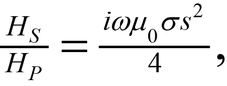
McNeill (1990) gives an excellent review and tutorial of electromagnetic methods, and much of his discussion on the terrain conductivity meter is excerpted here (see also Butler (1986)). He lists three significant differences between terrain conductivity meters and the traditional HLEM (horizontal loop electromagnetic) method usually used in mining applications. Perhaps the most important is that the operating frequency is low enough at each of the intercoil spacings that the electrical skin depth in the ground is always significantly greater than the intercoil spacing. Under this condition (known as operating at low induction numbers), virtually all response from the ground is in the quadrature phase component of the received signal. With these constraints, the secondary magnetic field can be represented as
 (1)
(1)
where
HS = secondary magnetic field at the receiver coil
HP = primary magnetic field at the receiver coil
Ω = 2πf
f = frequency in Hz
μ0 = permeability of free space
σ = ground conductivity in S/m (mho/m)
s = intercoil spacing in m
I = (-1)1/2, denoting that the secondary field is 90° out of phase with the primary field
Thus, for low and moderate conductivities, the quadrature phase component is linearly proportional to ground conductivity, so the instruments read conductivity directly (McNeill 1980). Given HS/HP , the apparent conductivity indicated by the instrument is defined as
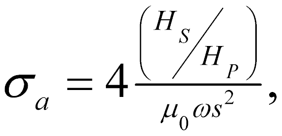 (2)
(2)
The low induction number condition also implies that the measured signals are of extremely low amplitude. Because of the low amplitude signals, terrain conductivity meters must have detection electronics that are an order of magnitude more sensitive than conventional HLEM systems.
The second difference is that terrain conductivity instruments are designed so that the quadrature phase zero level stays constant with time, temperature, etc., to within about 1 millisiemen/meter (mS/m). The stability of this zero level means that at moderate ground conductivity, these devices give an accurate measurement of bulk conductivity of the ground. These devices, like the conventional HLEM system, do not indicate conductivity accurately in high resistivity ground, because the zero error becomes significant at low values of conductivity.
The third difference is that operation at low induction numbers means that changing the frequency proportionately changes the quadrature phase response. In principle and in general, either intercoil spacing or frequency can be varied to determine variation of conductivity with depth. However, in the EM-31, EM-34, and EM‑38 systems, frequency is varied as the intercoil spacing is varied. Terrain conductivity meters are operated in both the horizontal and vertical dipole modes. These terms describe the orientation of the transmitter and receiver coils to each other and the ground, and each mode gives a significantly different response with depth as shown in figure 4. Figure 5 shows the cumulative response curves for both vertical dipoles and horizontal dipoles. These curves show the relative contribution to the secondary magnetic field (and hence apparent conductivity) from all material below a given depth. As an example, this figure shows that for vertical dipoles, all material below a depth of two intercoil spacings yields a relative contribution of approximately 0.25 (25%) to the response, i.e., the conductivity measurement. Thus, effective exploration depth in a layered earth geometry is approximately 0.25 to 0.75 times the intercoil spacing for the horizontal dipole mode and 0.5 to 1.5 for the vertical dipole mode. The commonly used systems use intercoil spacings of 1 m, 3.66 m, 10 m, 20 m, and 40 m.
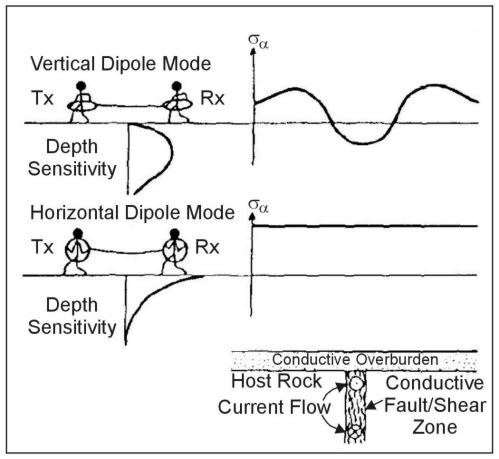
Figure 4. Terrain conductivity meter response over conductive dike. (McNeill 1990; copyright permission granted by Society of Exploration Geophysicists)
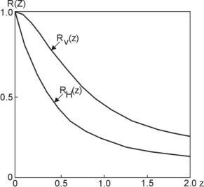
Figure 5. Cumulative response curves for both vertical coplanar and horizontal coplanar dipoles. Z is actually depth/intercoil spacing. (McNeill 1980; copyright permission granted by Geonics Ltd)
Terrain conductivity meters have shallower exploration depths than conventional HLEM, because maximum intercoil spacing is 40 m for the commonly used instruments. However, terrain conductivity meters are being widely used in geotechnical and environmental investigations. Of particular interest is the fact that when used in the vertical dipole mode, the instruments are more sensitive to the presence of relatively conductive, steeply dipping structures, whereas in the horizontal dipole mode the instruments are quite insensitive to this type of structure and can give accurate measurement of ground conductivity in close proximity to them.
Phase and other information are obtained in real time by linking the transmitter and receiver with a connecting cable. The intercoil spacing is determined by measuring the primary magnetic field with the receiver coil and adjusting the intercoil spacing so that it is the correct value for the appropriate distance. In the vertical dipole mode, the instruments are relatively sensitive to intercoil alignment, but much less so in the horizontal dipole mode. Terrain conductivity is displayed on the instrument in mS/m. (A conductivity of 1 mS/m corresponds to a resistivity of 1 kΩm or 1,000 Ωm.)
Data Interpretation
Because terrain conductivity meters read directly in apparent conductivity and most surveys using the instrument are done in the profile mode, interpretation is usually qualitative and of the "anomaly finding" nature. That is, the area of interest is surveyed with a series of profiles with a station spacing dictated by the required resolution and time/economics consideration. Typical station spacings are one-third to one-half the intercoil spacing. Any anomalous areas are investigated further with one or more of the following: other types of EM, resistivity sounding, other geophysical techniques, and drilling. Limited information about the variation of conductivity with depth can be obtained by measuring two or more coil orientations and/or intercoil separations and using one of several commercially available computer programs. The maximum number of geoelectric parameters, such as layer thicknesses and resistivities, which can be determined, is less than the number of independent observations. The most common instrument uses three standard intercoil distances (10, 20, and 40 m) and two intercoil orientations, which results in a maximum of six observations. Without other constraints, a two-layer model is the optimum.
Example 1 - Mapping Industrial Groundwater Contamination. Non-organic (ionic) groundwater contamination usually results in an increase in the conductivity of the groundwater. For example, in a sandy soil, the addition of 25 ppm of ionic material to groundwater increases ground conductivity by approximately 1 mS/m. The problem is to detect and map the extent of the contamination in the presence of conductivity variations caused by other parameters such as changing lithology. Organic contaminants are generally insulators and thus tend to reduce the ground conductivity, although with much less effect than an equivalent percentage of ionic contaminant. Fortunately, in many cases where toxic organic substances are present, there are ionic materials as well, and the plume is mapped on the theory that the spatial distribution of both organic and ionic substances is essentially the same, a fact that must be verified by subsequent sampling from monitoring wells installed on the basis of the conductivity map.
McNeill (1990) summarizes a case history by Ladwig (1982) that uses a terrain conductivity meter to map the extent of acid mine drainage in a rehabilitated surface coal mine in Appalachia. Measurements were taken with an EM ground conductivity meter in the horizontal dipole mode at both 10- and 20-m intercoil spacings (10-m data are shown in figure 6). Ten survey lines, at a spacing of 25 m, resulted in 200 data points for each spacing; the survey took 2 days to complete. In general, conductivity values of the order of 6 to 10 mS/m are consistent with a porous granular material reasonably well-drained or containing nonmineralized groundwater. Superimposed on this background are two steep peaks (one complex) where conductivities rise above 20 mS/m.
Wells F, G, and X were the only wells to encounter buried refuse (well W was not completed), and all three are at or near the center of the high conductivity zones. The water surface at well F is about 3 m below the surface, and at well X is 16.2 m below the surface. In fact, the only region where the water surface is within 10 m of the surface is at the southern end of the area; the small lobe near well D corresponds to the direction of groundwater flow to the seep (as the result of placement of a permeability barrier just to the west of the well). It thus appears that in the area of wells X and W, where depth to water surface is large, the shape and values of apparent conductivity highs are due to vertically draining areas of acidity. Further to the south, the conductivity high is probably reflecting both increased acidity and proximity of the water surface.
Examples 2 And 3 - Mapping Soil And Groundwater Salinity. EM techniques are well suited for mapping soil salinity to depths useful for the agriculturalist (the root zone, approximately 1 m), and many salinity surveys have been carried out with EM ground conductivity meters (McNeill 1990). In arid areas where the water surface is near the surface (within a meter or so), rapid transport of water to the surface as a result of capillary action and evaporation takes place, with the consequence that dissolved salts are left behind to hinder plant growth (McNeill 1986).
An EM terrain conductivity meter with short intercoil spacing (a few meters or less) is necessary to measure shallow salinity. Fortunately, the values of conductivity, which result from agriculturally damaging salinity levels, are relatively high, and interfering effects from varying soil structure, clay content, etc., can usually be ignored. Equally important, because salt is hygroscopic, those areas that are highly salinized seem to retain enough soil moisture to keep the conductivity at measurable levels even when the soil itself is relatively dry.
McNeill (1990) summarizes the results of a high-resolution survey of soil salinity carried out by Wood (1987) over dry farm land in Alberta, Canada (figure 7). For this survey, an EM terrain conductivity meter with an intercoil spacing of 3.7 m was mounted in the vertical dipole mode on a trailer, which was, in turn, towed behind a small four-wheeled, all-terrain vehicle. The surveyed area is 1,600 m long by 750 m wide. The 16 survey lines were spaced 50 m apart resulting in a total survey of 25 line km, which was surveyed in about 7 hr at an average speed of 3.5 km/hour. Data were collected automatically every 5.5 m by triggering a digital data logger from a magnet mounted on one of the trailer wheels.
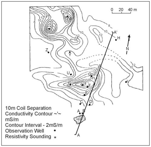
Figure 6. Contours of apparent conductivity for an acid
mine dump site in Appalachia from terrain conductivity meter.
(Ladwig (1982) and McNeill (1990); copyright permission granted
by Society of Exploration Geophysicists)
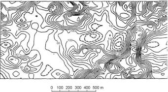
Figure 7. Contours of apparent conductivity measured with ground conductivity meter over dry farm land. Alberta, Canada. (Wood (1987) in McNeill (1990); copyright permission granted by Society of Exploration Geophysicists)
Survey data are contoured directly in apparent conductivity at a contour interval of 20 mS/m. The complexity and serious extent of the salinity is quite obvious. The apparent conductivity ranges from a low of 58 mS/m, typical of unsalinized Prairie soils, up to 300 mS/m, a value indicating extreme salinity. Approximately 25% of the area is over 160 mS/m, a value indicating a high level of salinity. The survey revealed and mapped extensive sub-surface salinity, not apparent by surface expression, and identified the areas most immediately threatened.
An example of a deeper penetrating survey to measure groundwater salinity was conducted by Barker (1990). The survey illustrates the cost-effective use of electromagnetic techniques in the delineation of the lateral extent of areas of coastal saltwater intrusion near Dungeness, England. As with most EM profiling surveys, a number of resistivity soundings were first made at the sites of several drill holes to help design the EM survey. In figure 8, a typical sounding and interpretation shows a three-layer case in which the low resistivity third layer appears to correlate with the conductivity of water samples from the drill holes and the clay/ sand lithology. To achieve adequate depth of investigation so that changes in water conductivity within the sands would be clearly identified, large coil spacings of 20 and 40 m were employed. The area is easily accessible and measurements can be made rapidly, but to reduce errors of coil alignment over some undulating gravel ridges, a vertical coil configuration was employed. This configuration is also preferred as the assumption of low induction numbers for horizontal coils breaks down quickly in areas of high conductivity. The extent of saline groundwater is best seen on figure 9, which shows the contoured ground conductivity in mS/m for the 40-m coil spacing. This map is smoother and less affected by near-surface features than measurements made with the 20-m coil spacing, and shows that the saline intrusion generally occurs along a coastal strip about 0.5 km wide. Flooding of inland gravel pits by the sea has allowed marine incursion in the west, leaving an isolated body of fresh water below Dungeness.
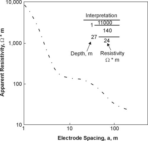
Figure 8. Typical resistivity sounding and interpretation, Dungeness, England. (Barker 1990; copyright permission granted by Society of Exploration Geophysicists)
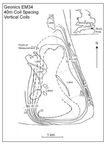
Figure 9. Contours of ground conductivity in mS/m, Dungeness, England. (Baker 1990; copyright permission granted by Society of Exploration Geophysicists)
Example 4 - Subsurface Structure. Dodds and Ivic (1990) describe a terrain conductivity meter survey to investigate the depth to basement in southeast Australia. During the first part of the survey, time domain EM and resistivity soundings were used to detect a basement high, which impedes the flow of saline groundwater. In the second part of the survey, a terrain conductivity meter was used to map the extent of the basement high as far and as economically as possible. The largest coil separation available with the instrument, 40 m, was used to get the deepest penetration with horizontal coil orientation. A very limited amount of surveying, using short traverses, successfully mapped out a high-resistivity feature (figure 10). This zone is confirmed by the plotted drilling results.
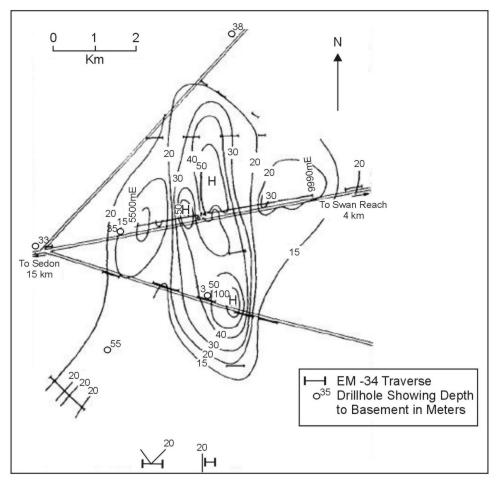
Figure 10. Apparent conductivity contours in ohm-m from a terrain conductivity meter survey in southern Australia. (Dodds and Ivic 1990; copyright permission granted by Society of Exploration Geophysicists).
The pages found under Surface Methods and Borehole Methods are substantially based on a report produced by the United States Department of Transportation:
Wightman, W. E., Jalinoos, F., Sirles, P., and Hanna, K. (2003). "Application of Geophysical Methods to Highway Related Problems." Federal Highway Administration, Central Federal Lands Highway Division, Lakewood, CO, Publication No. FHWA-IF-04-021, September 2003. http://www.cflhd.gov/resources/agm/