
Geophysical Methods
Electromagnetic Methods
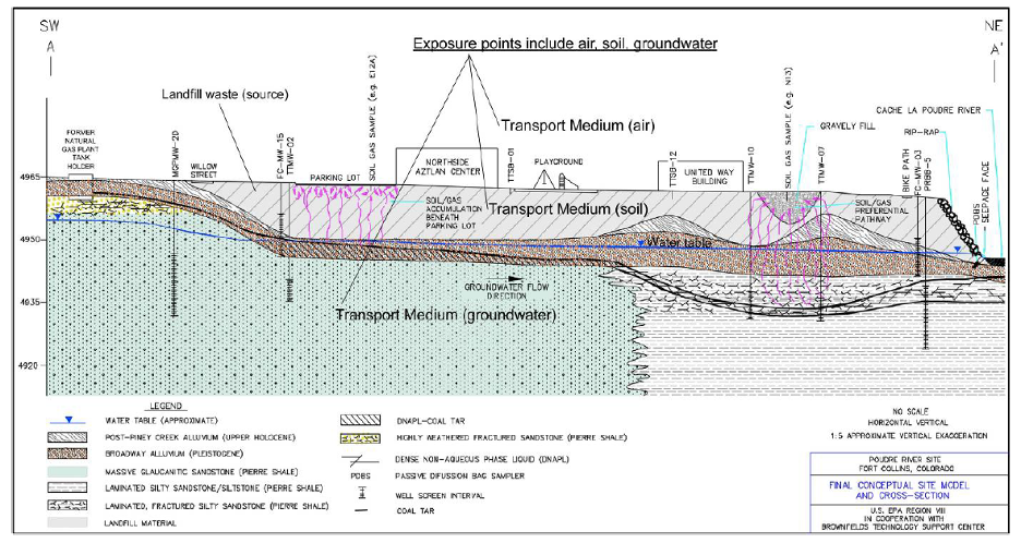
Figure 1. This CSM cross-section was developed using electromagnetic and resistivity geophysical surveys and other characterization tools (soil boring logs, soil gas surveys, groundwater sampling) to define subsurface conditions across the site. This includes the bedrock surface and fractures, subsurface channels in alluvium, and underground utilities that might act as preferential pathways (EPA, 2008![]() ).
).
Electromagnetic induction (EMI) methods use lower frequency radio waves and audio portions of the electromagnetic (EM) spectrum to characterize variability in the apparent electrical conductivity of subsurface materials. According to Everett (2013), the response recorded by the EM induction method is almost entirely due to the bulk subsurface electrical conductivity. Various configurations of EMI instrumentation can be applied for use in environmental site characterization, contaminated soil and groundwater investigations, mineral exploration, or water resources exploration (Doolittle and Brevik, 2014). EMI can be used to detect geologic and hydrogeologic conditions such as depth to bedrock or other geologic contacts, preferential pathways (such as faults, fractures, and voids), saltwater intrusion, and aquifer recharge, as well as environmental conditions such as light nonaqueous phase liquid (LNAPL) and dense nonaqueous phase liquid (DNAPL) thickness, acid mine drainage, landfill seepage (leachate), and buried drums (EPA, 1988, 1993, 1994; ASTM 2018). EMI can be used in conjunction with other characterization tools at contaminated sites to develop a conceptual site model (CSM) that visually represents subsurface conditions (Figure 1). A CSM helps narrow the focus of additional site investigations and provides a basis for the design of remedial actions (EPA, 2008![]() ). EMI measurements are collected by time-domain1 (TDEM) or frequency domain2 (FDEM) instrumentation deployed on the ground surface, in open boreholes, or via airborne techniques depending on the scale of study.
). EMI measurements are collected by time-domain1 (TDEM) or frequency domain2 (FDEM) instrumentation deployed on the ground surface, in open boreholes, or via airborne techniques depending on the scale of study.
Typical Uses
During site investigations, EMI tools can be used to (Stanford University, 2021):
- Map soil types.
- Map lateral changes in geology.
- Identify and map faults.
- Detect and map contaminant plumes.
- Detect groundwater seeps.
- Identify buried drums, tanks, metal utilities, and other metal objects.
For surface EMI tools, the depths of investigation depend on the coil spacing (0.5 to 60 meters) and frequencies used, but in general, investigation depths can range from sub-meter to 1,000 meters, depending on the equipment used (EPA, 1988, 2008). For borehole EMI tools, measurements are typically recorded 16 inches into the formation as described in the USGS Fractured Rock Geophysical Toolbox Method Selection Tool (2016). For airborne tools, the depth of investigation ranges from just a few meters to approximately 300 meters depending upon the configuration of the coil spacing and frequencies used (Ball, et al., 2011![]() ;USGS, 2016
;USGS, 2016![]() ).
).
Theory of Operation
EM tools use a transmitter coil to generate an electrical current that produces a primary electromagnetic field. Material (can be soil/rock, groundwater, or buried objects) in the subsurface interacts with this primary field to produce a secondary electromagnetic field that is detected and measured by a receiver coil (Doolittle and Brevik, 2014; Munnaf et al. 2020).
TDEM measures the change in response as time passes after the transmitted signal is abruptly turned off, and FDEM records the response in the subsurface as the electromagnetic field is transmitted at different frequencies.
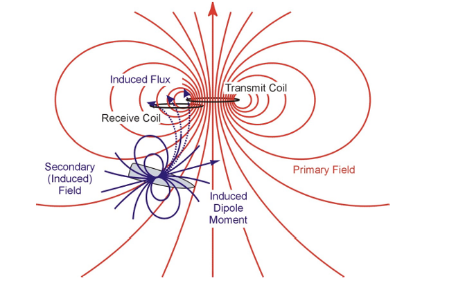
Figure 2. Primary fields (in red) are created by a transmitter coil. These primary fields generate secondary fields (blue) in the material that are detected by the receiver coil (USACE, 2016).
FDEM induces eddy currents in the subsurface as the transmitter coil creates a sinusoidal electromagnetic field. The primary and secondary electromagnetic fields generated by the eddy current loops are intercepted by the receiver coil to produce a voltage that is linearly related to the subsurface conductivity. This measurement is the cumulative sum of the variations in the electromagnetic properties of the material from the surface to the effective depth of the instrument (EPA, 1993).
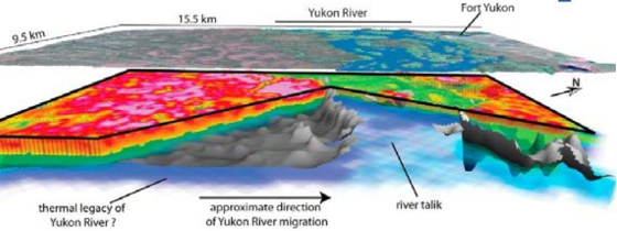
Figure 3. 3-Dimensional FDEM data. The upper plane is a Landsat view of the region displayed below. Higher resistivities are shown in warmer colors, and lower resistivities, like saturated material, are shown in blue and green (USACE, 2016).
Figure 2 illustrates how secondary fields are generated by metallic objects such as unexploded ordnance (UXO). If the subsurface target is a distributed conductivity medium such as a geologic formation, the entire medium produces the secondary fields (USACE, 2016).
FDEM measurements can be collected via airborne, surface-based, or waterborne systems to provide spatially continuous data of variations in subsurface electromagnetic properties. For quantitative evaluations of the subsurface resistivity structures, the data must be inverted (Figure 3) to produce a distribution of resistivity values with depth (USACE, 2016).
The effective depth of the FDEM instrument depends on the geometry and spacing of the transmitting and receiving coils and the frequency of EM field generated. Deeper target depths can be achieved by greater spacing between the transmitter and receiver coils or by using lower frequency EM fields. The closer the transmitter and coils are spaced together, the higher the data resolution (EPA, 1993![]() ; ITRC, 2019
; ITRC, 2019![]() ).
).
To measure TDEM, a single-turn square transmitter loop is laid on the ground with the receiver coil placed nearby. A steady current generated by the transmitter initially flows through the loop, and then is abruptly shut off. The eddy current descends to greater depths in the subsurface. As the current descends, the magnetic field decays. The measured decay in magnetic field provides the resistivity of the subsurface as a function of depth. The instrument's exploration depth, ranging from a few to about 300 meters, is determined by the product of the current and the area of the transmitter, the time it takes for the magnetic field to decay, and the configuration (orientation, geometry, and spacing) of the transmitter and receiver loops (EPA, 1993, ITRC, 2019![]() ).
).
System Components
The system components depend on the mode of deployment (by air, on ground surfaces, or in boreholes) of the EMI tools.
FDEM System Components
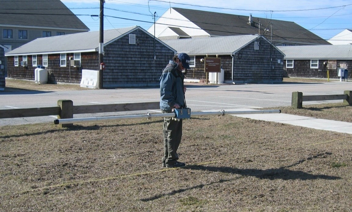
Figure 4. Operator uses a handheld surface EMI tool to collect FDEM data. The transmitter and receiver coils are located on opposite ends of the tool (USGS, 2008).
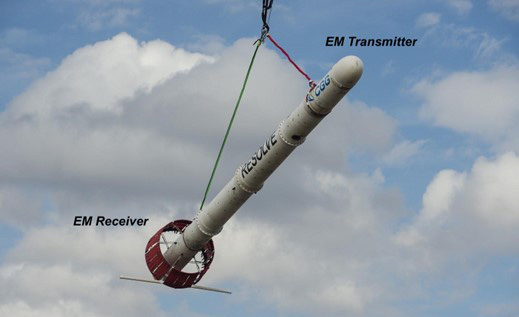
Figure 5. An example of the equipment used to collect airborne FDEM data (USGS).
During surface-based FDEM measurements, the receiver and transmitter coils are connected to a power source that generates the signal emitted by the transmitter. The housing for the power source contains a data logger that records the receiver coil's response to the electromagnetic field created by the transmitter coil. An example of a handheld surface tool used to collect FDEM measurements is shown in Figure 4.
Figure 5 shows a "bird," the cigar-shaped, 9-meter-long tube housing the electromagnetic sensor used to collect airborne FDEM measurements. The receiver and transmitter are located on opposite ends of the bird, which is suspended beneath a helicopter. The data logger is usually on board the helicopter.
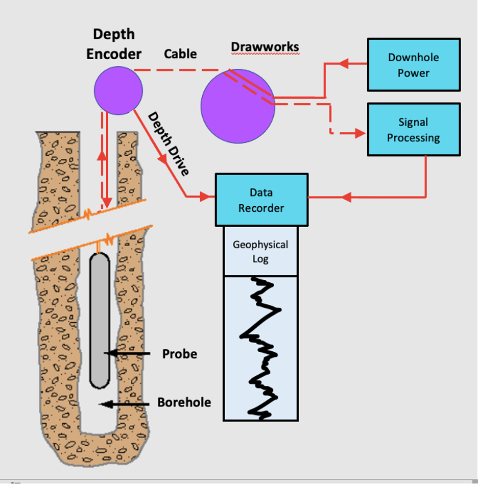
Figure 6. Schematic of a geophysical logging system, including a probe, cable and pulleys/winches, power and processing modules, and data recording units (U.S. Geological Survey, 2000).
When deployed in boreholes, an FDEM induction probe is attached to a geophysical logging system (Figure 6). The transmitter and receiver coils are located on either end of the probe and connected to a surface data logger by a cable (Williams et al., 1993).
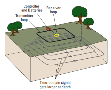
Figure 7. Setup of time-domain electromagnetic surface-geophysical equipment. The TDEM equipment is set up directly on the ground (USGS, 2021![]() ).
).
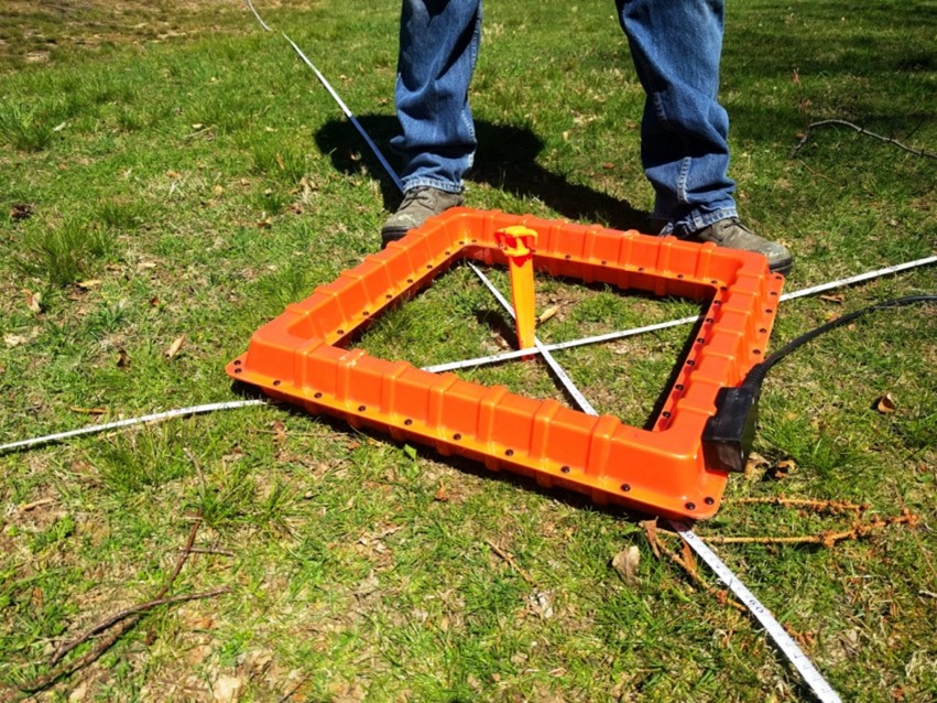
Figure 8. Photograph of a TDEM receiver coil (USGS, 2017).
TDEM System Components
Figure 7 illustrates the setup of TDEM equipment on the ground surface. The transmitter loop is laid on the ground in a rectangular shape, and the receiver coil is placed within the transmitter loop; then a data logger and power source are attached to the setup. Figure 8 shows an example of the receiver coil for a surface TDEM survey.
Airborne TDEM surveys use a hexagonal "hoop" configuration suspended below a helicopter (Figure 9). The transmitter and receiver coils are located on opposite ends of the hoop.
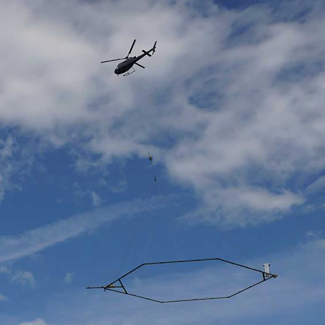
Figure 9. Helicopter towing a geophysical device as part of an electromagnetic and magnetic survey to collect TDEM data (USGS).
Modes of Operation
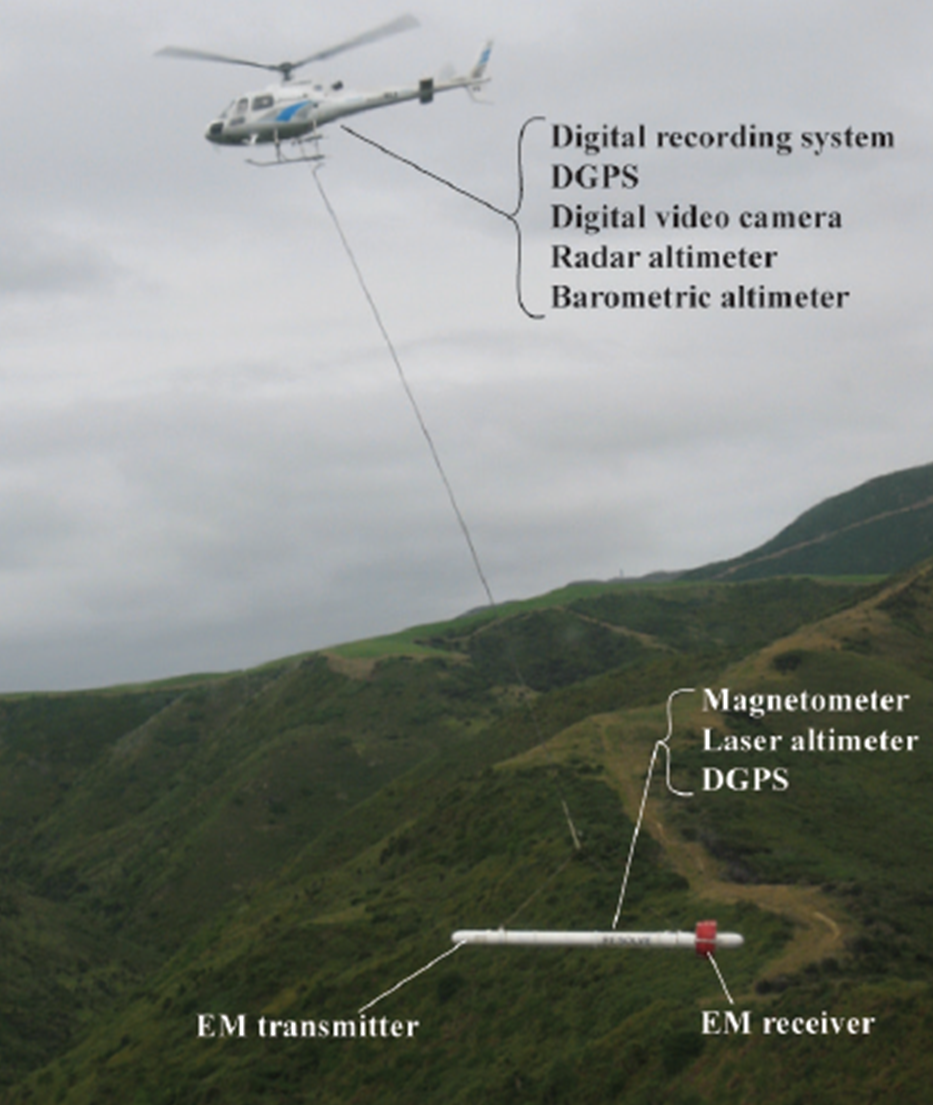
Figure 10. Helicopter-borne RESOLVE geophysical system used to collect FDEM data. The cylindrical shaped 'bird' contains the sensors (Ball, et al., 2011![]() ).
).
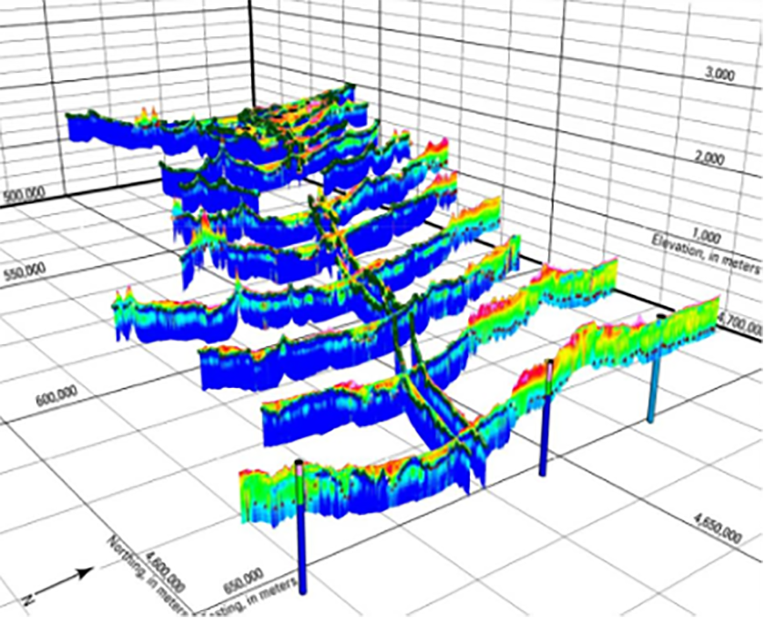
Figure 11. 3-Dimensional data projection of inverted time-domain electromagnetic data and airborne electromagnetic sections from an airborne survey of the North Platte Natural Resources District (USGS, 2011![]() ).
).
Airborne EMI (AEM) Surveys — In AEM surveys, geophysical instruments are suspended below a helicopter in either a "bird" configuration (Figure 10) to collect FDEM data or a hoop configuration to collect TDEM data. An electromagnetic signal is created by a current generated in the hoop or bird that transmits into the subsurface. A receiver mounted on the hoop or bird measures the response of the subsurface materials to the signal. For FDEM data, the response depends on the frequency, coil orientation, system elevation above ground surface, and the electrical resistivity of the subsurface. Depth images can be constructed using multiple coil pairs (transmitter and receiver) that measure at different frequencies (Ball, et al., 2011![]() ). In general, higher frequencies yield depths of investigation of just a few meters, while lower frequencies can reach up to 300 meters (Ball, et al., 2011
). In general, higher frequencies yield depths of investigation of just a few meters, while lower frequencies can reach up to 300 meters (Ball, et al., 2011![]() and USGS, 2016
and USGS, 2016![]() ). Flight paths collect the data in a "lawn-mowing" pattern to provide complete coverage of an area. Data are processed to create cross-sectional slices and 3-dimensional images (Figure 11) of the subsurface (USGS, 2016
). Flight paths collect the data in a "lawn-mowing" pattern to provide complete coverage of an area. Data are processed to create cross-sectional slices and 3-dimensional images (Figure 11) of the subsurface (USGS, 2016![]() ).
).
Figure 12. A USGS hydrologist calibrating an electromagnetic induction borehole logging tool (USGS, 2008).
EMI Borehole Logging — EMI borehole logging uses an induction probe designed to fit within small diameter monitoring wells typically found at contaminated sites. The logs can be used in water-, air-, and mud-filled holes and holes cased with PVC. EMI logging tools collect conductivity data that varies based on the porosity, permeability, and clay content of the geologic material. In addition, the conductivity of subsurface water varies with dissolved solids content (U.S. Geological Survey). Figure 12 shows an EMI logging tool being calibrated before use in the field.
Surface EMI Surveys — Surface EMI surveys can collect either TDEM or FDEM data (Figure 13).
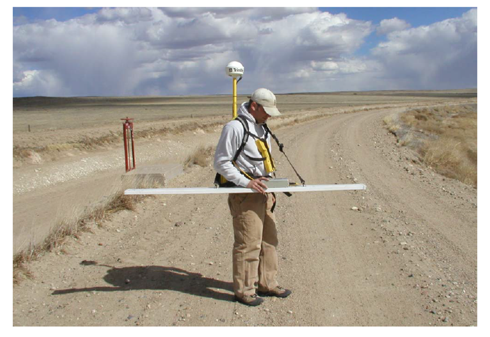
Figure 13. FDEM surface survey using a handheld EMI meter with fixed coils (Lucius, et al., 2006![]() ).
).
The meter has a fixed coil spacing that can measure several frequencies simultaneously by one person. The person then walks back and forth in a lawn-mower pattern, creating a broad 2-D areal image of the site at the depth of interest.
For instruments with separated coils (Figure 14), one person holds the receiver coil while the second person holds the transmitter coil (Lucius et al., 2006).
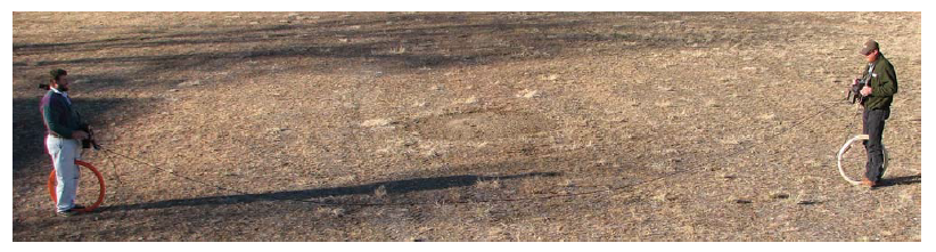
Figure 14. FDEM surface EMI survey using two separate coils (Lucius, et al., 2006![]() ).
).
Figure 15. USGS scientists setting up surface EMI survey equipment to collect TDEM data (USGS, 2016).
Surface EMI surveys that collect TDEM data require at least two people to set up and operate the equipment (Figure 15). Transmitter wire is laid on the ground surface within a large square that measures up to 300 feet across with the receiver system and data logger placed in the center. Once the setup is complete, a battery-generated electrical current is pulsed through the transmitter wire. The secondary EM fields are measured by the receiver and recorded on the data logger (USGS, 2017).
↩Data Display and Interpretation
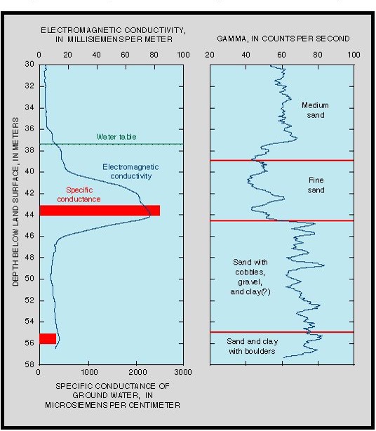
Figure 16. An example of an electromagnetic induction log recording the electrical conductivity of the geologic material and groundwater within the formation surrounding the borehole (USGS, 2000). Electromagnetic conductivity of the groundwater is shown by the blue line on the left side of the figure. Groundwater-specific conductance values (on the secondary horizontal axis) are shown in red bars and correspond to the most highly contaminated part of a leachate plume in a sand and gravel aquifer downgradient of a municipal landfill.
Borehole EMI Survey Data — Borehole EMI tools measure conductivity relative to depth in the formation immediately adjacent to the borehole. Porosity of the formation, permeability, clay content, and the dissolved-solids concentrations within the formation water affect the conductivity, which is presented in millisiemens per meter (mS/m). Figure 16 shows an example of a borehole log of EM conductivity with depth. The specific conductance corresponds to an increase in electromagnetic conductivity due to contamination caused by landfill leachate at a depth of approximately 44 meters (USGS, 2000).
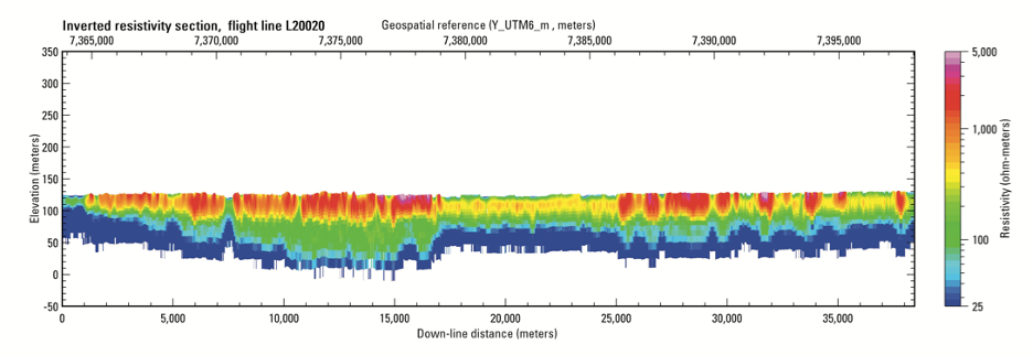
Figure 17. Inverted resistivity data from an airborne flight line. Warm colors indicate higher resistivity, and cool colors indicate lower resistivity (USGS, 2011![]() ).
).
FDEM Survey Data — An FDEM system collects the in-phase and out-of-phase response to the transmitted signal. The signals are processed to show apparent resistivity for each frequency, and a corresponding apparent depth is estimated. The apparent resistivity is an estimated parameter based on an assumed measurement and a homogeneous subsurface. Data are processed for system drift and calibrations and can be inverted with algorithms to depict the distribution of electrical resistivity with depth (Ball, et al., 2011). Figure 17 is an example of inverted data collected by an airborne survey.
TDEM Survey Data — A TDEM system transmits pulses of current into the subsurface. The raw data consist of measured amplitudes of the decaying electromagnetic field from each pulse. Collected data typically undergo a filtering and leveling process. Drift corrections are applied, and filters can be used to remove confounding effects from factors such as lightning. Lag-time corrections are applied to account for geometric offset between the navigational sensors on the helicopter and the electromagnetic sensors on the hoop. Data are inverted using a computer program to depict the distribution of resistivity with depth beneath each sounding (Bedrosian, et al., 2014![]() ). Figures 18 and 19 show post-processed TDEM data.
). Figures 18 and 19 show post-processed TDEM data.
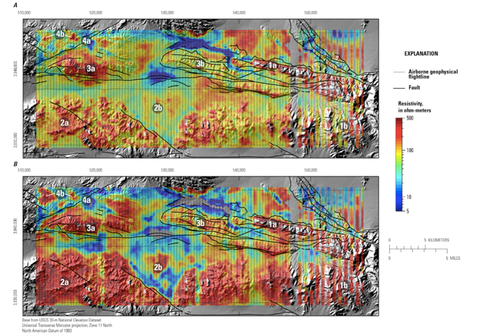
Figure 18. Post-processed TDEM data from a flight line showing depth slices through the inverted resistivity model at a depth of 25 meters (A) and 125 meters (B) (Bedrosian, et al., 2014![]() ).
).
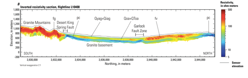
Figure 19. Example of inverted resistivity section along a flight line. The warm colors (red) indicate higher resistivity while the cool colors (blues) indicate lower resistivities, in this case the saturated zone (Bedrosian, et al., 2014![]() ).
).
Performance Specifications
Performance specifications for FDEM and TDEM instruments are summarized in the table below.
| Performance Specifications | ||
| Parameter | FDEM | TDEM |
| How it Works | Uses the magnitude and phase of the secondary field resulting from induced electromagnetic currents. | Measures secondary magnetic fields from decaying induced pulsed currents. |
| Mode of Operation | Ground-based, airborne, waterborne, borehole. | Airborne, ground-based, waterborne, borehole. Can also be adapted for use on ice2. |
| Primary Applications | Identify depth to bedrock, fractures and fault zones, voids and sinkholes, soil and rock properties, and saline intrusion, as well as buried drums, underground storage tanks (USTs), landfill boundaries, utilities, and conductive groundwater contamination1,3. | Depth and thickness of stratigraphy, fractures, depth to water table, depth to aquitard, presence of coastal or inland groundwater salinity, as well as detection and mapping of groundwater, inorganic plumes, seepage from brine pits, and salt-water intrusion1,2. |
| Depth | 0.75 to 60 m (2.5 to 200 ft), dependent on coil configuration3. | 6 to 1000 m (20 to 3000 ft) or more, dependent on instrument orientation2, 3. TDEM ground arrays allow for larger transmitter loops, hence increased measurement depths. |
| Unit of Measurement | SI units1: Conductivity: millisiemens per meter (mS/m) Intercoil spacing meters (m) Ratio of secondary magnetic field to primary magnetic field (Hs/Hp): unitless |
SI units2: Voltage: nanovolts per square meter (nV/m2) Resistivity: ohmmeters (Ω.m) Conductivity: millisiemens per meter (mS/m) |
| Precision | Changes in temperature, soil moisture, and electromagnetic noise, as well as small errors in location and coil alignment and spacing, will affect precision1. | Measurements are expected to be within 2 to 3 % of one another under identical conditions and low noise levels2. |
| Lateral Resolution | Lateral resolution determined by spacing between transmitter and receiver coils and spacing between measurements 1. Varies between 0.5- 10 m. | Lateral resolution determined by transmitter loop size and spacing between soundings; TDEM is unable to resolve small features that are spaced less than the spacing between stations1. |
| Vertical Resolution | Function of depth, thickness, conductivities and layer conductivity contrasts, and instrument used for the survey1. FDEM can typically resolve 2 to 3 lithologic or material layers1,3. | Function of targets, sizes, depths, relative positions, and resistivities1. TDEM can typically resolve 3 to 4 lithologic or material layers3. |
- ASTM 2018 (D6639-18) Standard Guide for Using the Frequency Domain Electromagnetic Method for Subsurface Site Characterizations.
- ASTM 2020a (D6820-20) Standard Guide for Use of the Time Domain Electromagnetic Method for Geophysical Subsurface Site Investigation.
- ASTM 2020b (D6429-20) Standard Guide for Selecting Surface Geophysical Methods.
Advantages
Advantages of EMI tools include (EPA, 1993 and USGS, 2016):
- Handheld EMI tools are physically manageable with 1-2 people.
- Handheld logging equipment has a resolution range of 0.5 to 10 meters.
- They are non-invasive.
- Airborne surveys can cover areas that are remote and less accessible.
- Borehole EMI can be used to monitor changes in subsurface properties over time.
Limitations
Limitations for EMI tools include (EPA, 1993 and USGS, 2016):
- Target must have contrasting electromagnetic properties between the area of interest relative to the non-targeted material.
- Some terrain is not easily accessible for handheld surveys.
- Borehole EMI cannot be used in steel-cased holes.
- Borehole EMI cannot determine the conductivity of thin beds.
- EMI methods are susceptible to interference from metal, power lines, and other factors.
- Conductive overburden can limit the depth of exploration for surface EMI tools.
- Airborne surveys can be expensive.
Cost
Costs vary significantly depending upon the mode of operation and the type of survey conducted. Rental costs for a single-person operated surface electromagnetic instrument can range from $200 to $500 (USD)/week. For airborne surveys, the rental costs range from $48.27 (USD) per mile to roughly $1,600 (USD) per mile (OpenEI). For an FDEM survey, a single operator can complete two to three acres (with five foot or greater line spacing) per day under favorable conditions. Data acquisition costs range from $2,000 to $3,000 (USD) per day depending on the type of instrument and site conditions (ITRC, 2019). For airborne TDEM surveys, costs range from $16,000 to $25,000 (USD) per day. Costs for a ground survey range from $1,800 to $5,000 (USD) per day (ITRC, 2019). Costs to purchase surface TDEM survey equipment range from $45,000 to $65,000 (USD), and surface FDEM survey equipment ranges from $20,000 to $30,000 (USD) (Lucius, et al., 2006![]() ).
).
Case Studies
![]() Airborne Electromagnetic and Magnetic Geophysical Survey Data of the Yukon Flats and Fort Wainwright Areas, Central Alaska, June 2010
Airborne Electromagnetic and Magnetic Geophysical Survey Data of the Yukon Flats and Fort Wainwright Areas, Central Alaska, June 2010
Ball, L., et al., 2011.
Open-File Report 2011-1304, 21 pp.
The 3-dimensional distribution of permafrost was estimated using airborne electromagnetic and magnetic data collected by USGS in central Alaska. The effectiveness of the geophysical methods in mapping the permafrost was evaluated. The data were also used to better understand the subsurface physical properties in the areas of discontinuous permafrost.
![]() Airborne Electromagnetic Data and Processing Within Leach Lake Basin, Fort Irwin, California
Airborne Electromagnetic Data and Processing Within Leach Lake Basin, Fort Irwin, California
Bedrosian, P., et al., 2014.
Open-File Report 2013-1024-G, 20 pp.
Airborne electromagnetic (EM) and magnetic surveys were used to collect data to characterize the subsurface and provide information to manage groundwater resources in the Fort Irwin area. In addition to the airborne surveys, ground-based time-domain EMI soundings, laboratory resistivity measurements, and borehole geophysical logs from nearby basins were used to develop the resistivity stratigraphy for the area.
Frequency Domain Electromagnetic Method (FDEM) as a Tool to Study Contamination at the Sub-Soil Layer
Goldshleger, N., et al., 2019.
Geosciences, 9:9, 382, August.
Traditional sheep and cattle grazing has led to potential contaminant impacts to subsurface soil from buildup of animal waste products. The frequency domain electromagnetic method (FDEM) was used to characterize the soil salinity. The results show a correlation between the laboratory soil analysis and the FDEM analysis of soils.
Integrating Surface and Borehole Geophysics in the Characterization of Salinity in a Coastal Aquifer
Paillet, F., 2014.
Flow in the surficial aquifer near Big Cypress National Preserve in South Florida was characterized using geologic core descriptions, borehole geophysics, surface geophysical soundings, and water-sample analyses. Aquifer tests and piezometer measurements showed that the surficial aquifer is under unconfined conditions and in hydraulic connection with surface water bodies.
![]() An Integrated Hydrogeologic and Geophysical Investigation to Characterize the Hydrostratigraphy of the Edwards Aquifer in an Area of Northeastern Bexar County, Texas
An Integrated Hydrogeologic and Geophysical Investigation to Characterize the Hydrostratigraphy of the Edwards Aquifer in an Area of Northeastern Bexar County, Texas
Shah, S., et al., 2008.
Scientific Investigations Report 2008-5181, 26 pp.
USGS in conjunction with the San Antonio Water System characterized the hydrostratigraphy and the hydrogeologic features of the Edwards Aquifer in northeastern Bexar County, Texas. Existing information on the hydrostratigraphy was used along with local-scale geologic mapping and surface-based geophysical methods to identify ranges of electrical resistivity hydrostratigraphic zones within the Edwards Aquifer.
Application of Integrated Methods in Mapping Waste Disposal Areas
Soupios et al., (2007).
This paper discusses the use of environmental methods including electromagnetic conductivity, to characterize the hydrogeological, geological, and tectonic regime of the largest waste disposal landfill of Crete Island, the Fodele municipal solid waste site.
![]() Use of Time Domain Electromagnetic Soundings and Borehole Electromagnetic Induction Logs to Delineate the Freshwater/Saltwater Interface on Southwestern Long Island, New York, 2015-17
Use of Time Domain Electromagnetic Soundings and Borehole Electromagnetic Induction Logs to Delineate the Freshwater/Saltwater Interface on Southwestern Long Island, New York, 2015-17
Stumm, F., et al., 2020.
Open-File Report 2020-1093. 27 pp.
USGS and the New York State Department of Environmental Conservation delineated the freshwater/saltwater interface in the coastal plain aquifers in southwestern Long Island using surface and borehole geophysical methods. Extensive saltwater intrusion was documented for the first time.
Surface-Geophysical Investigation of the University of Connecticut Landfill, Storrs, Connecticut
USGS, 1999.
USGS in cooperation with the University of Connecticut conducted a surface-geophysical investigation of a landfill, chemical waste disposal pits, and the surrounding areas using surface-geophysical methods to measure geophysical anomalies that might indicate potential contamination or pathways for contamination.
Application of Electromagnetic Logging to Contamination Investigations in Glacial Sand-and-Gravel Aquifers
Williams, J., et al., 1993.
Groundwater Monitoring & Remediation, Vol. 13, Issue 3, pp 129-138. August.
EM, gamma, and lithologic logs, as well as specific conductance data from five sites in the northeastern U.S., were evaluated to assess the relationship between EM conductivity, aquifer lithology, and water quality in sand-and-gravel aquifers. The dissolved solids concentration of groundwater and the silt and clay content of the aquifer were the primary hydrogeologic factors that affected the EMI log response at the five sites.
↩References:
ASTM, 2018. Standard Guide for Using the Frequency Domain Electromagnetic Method for Subsurface Site Characterizations. Designation: D6639-18.
ASTM, 2020. Standard Guide for Use of the Time Domain Electromagnetic Method for Geophysical Subsurface Site Investigation. Designation: D6820-20.
ASTM 2020b. Standard Guide for Selecting Surface Geophysical Methods. Designation: D6429-20.
Ball, L., et al., 2011. Airborne Electromagnetic and Magnetic Geophysical Survey Data of the Yukon Flats and Fort Wainwright Areas, Central Alaska, June 2010![]() .
.
Open-File Report 2011-1304, 21 pp.
Bedrosian, P., et al., 2014. Airborne Electromagnetic Data and Processing Within Leach Lake Basin, Fort Irwin, California![]() .
.
Open-File Report 2013-1024-G, 20 pp.
Doolittle and Brevik, 2014. The Use of Electromagnetic Induction Techniques in Soils Studies.
EPA, 2008. Triad Issue Paper: Using Geophysical Tools to Develop the Conceptual Site Model![]() .
.
Office of Solid Waste and Emergency Response, 542-F-08-007, 15 pp. December.
EPA, 1994. Application Of Geophysics To Acid Mine Drainage Investigations, Volume 1: Literature Review and Theoretical Background![]() . California Department of Conservation Office of Mine Reclamation for Western Governors' Association. EPA 530-R-95-013a, 148 pp. September.
. California Department of Conservation Office of Mine Reclamation for Western Governors' Association. EPA 530-R-95-013a, 148 pp. September.
EPA, 1993. Use of Airborne, Surface, Borehole Geophysical Techniques at Contaminated Sites, A Reference Guide![]() . EPA/625/R-92/007, 304 pp. September.
. EPA/625/R-92/007, 304 pp. September.
EPA, 1988. Soil-Gas and Geophysical Techniques for Detection of Subsurface Organic Contamination![]() .
.
EPA/600/4-88/019, 88 pp. December.
Everett, M. E., 2013. Near-Surface Applied Geophysics. Cambridge: Cambridge University Press.
ITRC, 2019. Implementing Advanced Site Characterization Tools Team![]() , Report ASCT-1, 328 pp.
, Report ASCT-1, 328 pp.
Lucius, J., et al., 2006. An Introduction to Using Surface Geophysics to Characterize Sand and Gravel Deposits![]() .
.
Munnaf et al. 2020. Site-specific Seeding Using Multi-sensor and Data Fusion Techniques: A Review.
Open-File Report 2006-1257. 51 pp.
OpenEI, 2021. Exploration Technique: Electromagnetic Techniques. Website consulted July 2021.
OpenEI, 2021. Exploration Technique: Electromagnetic Techniques. Website consulted July 2021.
Schlumberger, 2021. Oilfield Glossary. Website consulted July 2021.
Shah, S., et al., 2008. An Integrated Hydrogeologic and Geophysical Investigation to Characterize the Hydrostratigraphy of the Edwards Aquifer in an Area of Northeastern Bexar County, Texas.
Scientific Investigations Report 2008-5181, 26 pp.
Stanford University, 2021. Geophysical Equipment. School of Earth, Energy & Environmental Sciences. Website consulted July 2021.
U.S. Army Corps of Engineers, 1995. Geophysical Exploration for Engineering and Environmental Investigations![]() . EM 1110-1-1802. 208 pp. August 31.
. EM 1110-1-1802. 208 pp. August 31.
U.S. Army Corps of Engineers (USACE), 2016. Evaluation of Electromagnetic Induction (EMI) Resistivity Technologies for Assessing Permafrost Geomorphologies. ERDC/CRREL TR-16-12. 44 pp. August.
U.S. Geological Survey (USGS), 2000. Media-Images: Geophysical Logging System. Website consulted July 2021.
U.S. Geological Survey (USGS), 2000. Media-Images: Geophysical Logs — Electromagnetic-induction Log. Website consulted July 2021.
U.S. Geological Survey (USGS), 2008. Media-Images: Electromagnetic Survey. Website consulted July 2021.
U.S. Geological Survey (USGS), 2008. Media-Images: USGS Training on Borehole Geophysical Logging. Website consulted July 2021.
U.S. Geological Survey (USGS) in cooperation with the New York State Department of Environmental Conservation, 2021. Scientific Investigations Report![]() . 2021-5008, 38 pp.
. 2021-5008, 38 pp.
U.S. Geological Survey (USGS), 2016. USGS Fractured Rock Geophysical Toolbox Method Selection Tool. Website consulted July 2021.
U.S. Geological Survey (USGS), 2016. Yellowstone Volcano Observatory, Airborne Electromagnetic & Seismic Imaging FAQ![]() . November.
. November.
U.S. Geological Survey (USGS), 2017. Media-Images: Time-Domain Electromagnetic Receiver Coil. Website consulted July 2021.
U.S. Geological Survey (USGS), 2017. Press Release: Electromagnetic Surveys in the Sky and on Land Give a View of What's Below Earth's Surface. Website consulted July 2021.
U.S. Geological Survey (USGS), 2020. Enhanced Characterization of the Hydrogeologic Framework — Mississippi Alluvial Plain (MAP) Regional Water Availability Study. Website consulted July 2021.
U.S. Geological Survey (USGS), 2020. Press Release: Low-flying Helicopter Will Survey Northeast Wisconsin for Geologic Study. December.
U.S. Geological Survey (USGS), 2021. Borehole Geophysics. Website consulted July 2021.
U.S. Geological Survey (USGS), 2021. Media-Images: Time Domain Electromagnetic Method Diagrams. Website consulted July 2021.
U.S. Geological Survey (USGS), 2021. Media-Images: CGG RESOLVE in Flight. Website consulted July 2021.
U.S. Geological Survey (USGS), 2021. Media-Images: Airborne electromagnetic Survey, Northeastern Wisconsin, January 2021. Website consulted July 2021.
U.S. Geological Survey (USGS), 2011. Geological Survey in cooperation with the North Platte Natural Resources District, the South Platte Natural Resources District, and the Nebraska Environmental Trust. Scientific Investigations Report![]() . 2011—5219, 47 pp.
. 2011—5219, 47 pp.
Williams, J., et al., 1993. Application of Electromagnetic Logging to Contamination Investigations in Glacial Sand-and-Gravel Aquifers. Groundwater Monitoring & Remediation, Vol. 13, Issue 3, p 129-138. August.
Helpful Information
Measurements are expressed as a function of time (Schlumberger). ↩
Measurements are expressed as a function of time (Schlumberger). ↩
Measurements are expressed as a function of frequency, where frequency is the rate of repetition of wavelengths of electrical signals measured in cycles per second or hertz (Schlumberger). ↩
Measurements are expressed as a function of frequency, where frequency is the rate of repetition of wavelengths of electrical signals measured in cycles per second or hertz (Schlumberger). ↩