Environmental Geophysics
Electrical Methods
Basic Concept
Spontaneous potential (SP) is one of the oldest logging techniques. It employs very simple equipment to produce a log whose interpretation may be quite complex, particularly in freshwater aquifers. This complexity has led to misuse and misinterpretation of spontaneous potential (SP) logs for groundwater applications. The spontaneous potential log (incorrectly called self potential) is a record of potentials or voltages that develop at the contacts between shale or clay beds and a sand aquifer, where they are penetrated by a drill hole. The natural flow of current and the SP curve or log that would be produced under the salinity conditions given are shown in Figure 1.
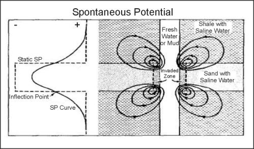
Figure 1. Flow of current at typical bed contacts and the resulting spontaneous potential curve and static values.
Data Acquisition
The SP measuring equipment consists of a lead or stainless steel electrode in the well connected through a millivolt meter or comparably sensitive recorder channel to a second electrode that is grounded at the surface (Figure 2). The SP electrode usually is incorporated in a probe that makes other types of electric logs simultaneously so it is usually recorded at no additional cost. Spontaneous potential is a function of the chemical activities of fluids in the borehole and adjacent rocks, the temperature, and the type and amount of clay present; it is not directly related to porosity and permeability. The chief sources of spontaneous potential in a drill hole are electrochemical, electrokinetic, or streaming potentials and redox effects. When the fluid column is fresher than the formation water, current flow and the SP log are as illustrated in Figure 1; if the fluid column is more saline than water in the aquifer, current flow and the log will be reversed. Streaming potentials are caused by the movement of an electrolyte through permeable media. In water wells, streaming potential may be significant at depth intervals where water is moving in or out of the hole. These permeable intervals frequently are indicated by rapid oscillations on an otherwise smooth curve. Spontaneous potential logs are recorded in millivolts per unit of t paper or full scale on the recorder. Any type of accurate millivolt source may be connected across the SP electrodes to provide calibration or standardization at the well. The volume of investigation of an SP sonde is highly variable, because it depends on the resistivity and cross‑sectional area of beds intersected by the borehole. Spontaneous potential logs are more affected by stray electrical currents and equipment problems than most other logs. These extraneous effects produce both noise and anomalous deflections on the logs. An increase in borehole diameter or depth of invasion decreases the magnitude of the SP recorded. Obviously, changes in depth of invasion with time will cause changes in periodic SP logs. Because the SP is largely a function of the relation between the salinity of the borehole fluid and the formation water, any changes in either will cause the log to change.
Data Interpretation
Spontaneous potential logs have been used widely in the petroleum industry for determining lithology, bed thickness, and the salinity of formation water. SP is one of the oldest types of logs, and is still a standard curve included in the left track of most electric logs. The chief limitation that has reduced the application of SP logs to groundwater studies has been the wide range of response characteristics in freshwater environments. As shown in Figure 1, if the borehole fluid is fresher than the native interstitial water, a negative SP occurs opposite sand beds; this is the so‑called standard response typically found in oil wells. If the salinities are reversed, then the SP response also will be reversed, which will produce a positive SP opposite sand beds. Thus, the range of response possibilities is very large and includes zero SP (straight line), when the salinity of the borehole and interstitial fluids are the same. Lithologic contacts are located on SP logs at the point of curve inflection, where current density is maximum. When the response is typical, a line can be drawn through the positive SP‑curve values recorded in shale beds, and a parallel line may be drawn through negative values that represent intervals of clean sand.
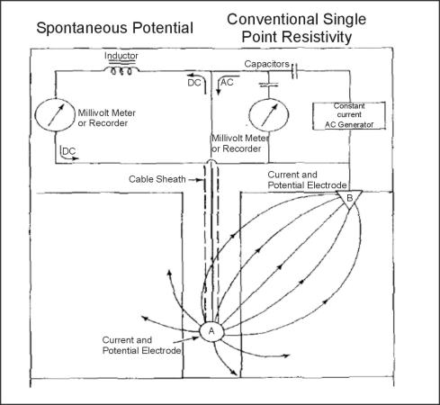
Figure 2. System used to make conventional single-point resistance spontaneous potential logs.
A typical response of an SP log in a shallow-water well, where the drilling mud was fresher than the water in the aquifers, is shown in Figure 3. The maximum positive SP deflections represent intervals of fine‑grained material, mostly clay and silt; the maximum negative SP deflections represent coarser sediments. The gradational change from silty clay to fine sand near the bottom of the well is shown by a gradual change on the SP log. The similarity in the acter of an SP log and a gamma log under the right salinity conditions also is shown in this figure. Under these conditions, the two types of logs can be used interchangeably for stratigraphic correlation between wells where either the gamma or the SP might not be available in some wells. The similarity between SP and gamma logs also can be used to identify wells where salinity relationships are different from those shown in Figure 360. Spontaneous‑potential logs have been used widely for determining formation-water resistivity (Rw) in oil wells, but this application is limited in fresh groundwater systems. In sodium chloride type saline water, the following relation is used to calculate Rw:
![]() (1)
(1)
where
SP = log deflection in mV,
K = 60 + 0.133T,
T = borehole temperature, in degrees Fahrenheit (metric and IP units are mixed for equation validity),
Rm = resistivity of borehole fluid, in Ohm-m,
Rw = resistivity of formation water, in ohm-m.
The SP deflection is read from a log at a thick sand bed; Rm is measured with a mud‑cell or fluid-conductivity log. Temperature may be obtained from a log, but it also can be estimated, particularly if bottom-hole temperature is available. The unreliability of determining Rw of fresh water using the SP equation has been discussed by Patten and Bennett (1963) and Guyod (1966). Several conditions must be met if the equation is to be used for groundwater investigations. These conditions are not satisfied in most freshwater wells. Both borehole fluids and formation water need to be sodium chloride solutions. The borehole fluid needs to be quite fresh, with a much higher resistivity than the combined resistivity of the sand and shale; this requirement usually means that the formation or interstitial water must be quite saline. The shales need to be ideal ion-selective membranes, and the sands need to be relatively free of clay. No contribution can be made to the SP from such sources as streaming potential.
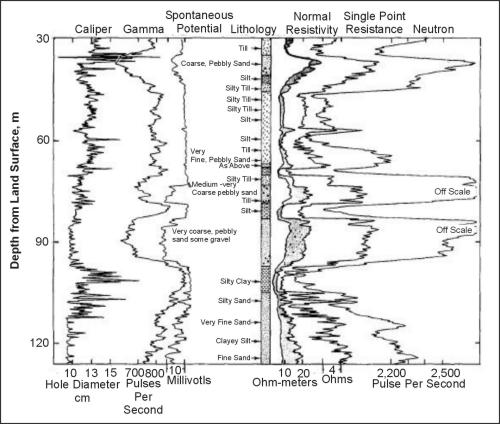
Figure 3. Caliper, gamma, spontaneous potential, normal resistivity, single point resistance and neutron logs compared to lithology; Kipling, Saskatchewan, Canda.
Basic Concept
The single‑point resistance log has been one of the most widely used in non‑petroleum logging in the past; it is still useful, in spite of the increased application of more sophisticated techniques. Single‑point logs cannot be used for quantitative interpretation, but they are excellent for lithologic information. The equipment to make single‑point logs usually is available on most small water‑well loggers, but it is almost never available on the larger units used for oil‑well logging. The resistance of any medium depends not only on its composition, but also on the cross‑sectional area and length of the path through that medium. Single‑point resistance systems measure the resistance, in W, between an electrode in the well and an electrode at the surface or between two electrodes in the well. Because no provision exists for determining the length or cross‑sectional area of the travel path of the current, the measurement is not an intrinsic acteristic of the material between the electrodes. Therefore, single‑point resistance logs cannot be related quantitatively to porosity, or to the salinity of water in those pore spaces, even though these two parameters do control the flow of electric current.
Data Acquisition
A schematic diagram of the equipment used to make conventional single‑point resistance and spontaneous potential logs is shown in Figure 2. The two curves can be recorded simultaneously if a two‑channel recorder is available. The same ground and down‑hole electrodes (A and B) are used for both logs. Each electrode serves as a current and as a potential sensing electrode for single‑point logs. The single‑point equipment on the right side of the figure actually measures a potential in volts (V) or mV, which can be converted to resistance by use of Ohm's law, because a constant current is maintained in the system. For the best single‑point logs, the electrode in the well needs to have a relatively large diameter, with respect to the hole diameter, because the radius of investigation is a function of electrode diameter. The differential system, with both current and potential electrodes in the probe, which are separated by a thin insulating section, provides much higher resolution logs than the conventional system but is not available on many loggers. Scales on single‑point resistance logs are calibrated in W per inch of span on the recorder. The volume of investigation of single‑point resistance sonde is small, approximately 5 to 10 times the electrode diameter. Single‑point logs are greatly affected by changes in well diameter, partly because of the relatively small volume of investigation.
Data Interpretation
Single-point resistance logs are useful for obtaining information on lithology; the interpretation is straightforward, with the exception of the extraneous effects described previously. Single-point logs have a significant advantage over multi-electrode logs; they do not exhibit reversals as a result of bed-thickness effects. Single-point logs deflect in the proper direction in response to the resistivity of materials adjacent to the electrode, regardless of bed thickness; thus, they have a very high vertical resolution. The response of both differential and conventional single-point logs to fractures is illustrated in figure 4. In this figure, at least one of the logging systems was not properly calibrated, because the scales differ by an order of magnitude. Hole enlargements shown on the caliper log are almost entirely caused by fractures in the crystalline rocks penetrated by this hole. The differential single-point log defines the fractures with much greater resolution than the log made with the conventional system.
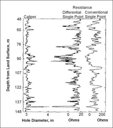
Figure 4. Caliper, differential and conventional single-point resistance logs in a well in fractured crystalline rocks.
Basic Concept
Among the various multi-electrode resistivity-logging techniques, normal resistivity is probably the most widely used in groundwater hydrology, even though the long normal log has become rather obsolete in the oil industry. Normal-resistivity logs can be interpreted quantitatively when they are properly calibrated in terms of Ώm. Log measurements are converted to apparent resistivity, which may need to be corrected for mud resistivity, bed thickness, borehole diameter, mudcake, and invasion, to arrive at true resistivity. ts for making these corrections are available in old logging manuals. Figure 5 is an example of one of these ts that is used to correct 40-cm (16-cm) in normal curves for borehole diameter and mud resistivity. The arrows on this t show examples of corrections for borehole size and mud resistivity (Rm). If the resistivity from a 40-cm (16-in) normal curve divided by the mud resistivity is 50 in a 25-cm (10-in) borehole, the ratio will be 60 in an 20cm (8-in) borehole. If the apparent resistivity on a 40-cm (16-in) normal log is 60 Ώm and the Rm is 0.5 Ώm in a 23-cm (9-in) well, the ratio on the X-axis is 195. The corrected log value is 97.5 Ώm at formation temperature. Temperature corrections and conversion to conductivity and to equivalent sodium chloride concentrations can be made using figure 6. To make corrections, the user should follow along isosalinity lines because only resistivity or conductivity change as a function of temperature, not ionic concentrations.
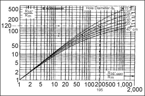
Figure 5. Borehole correction t for 16-in normal resistivity log. (copyright permission granted by Schlumberger)
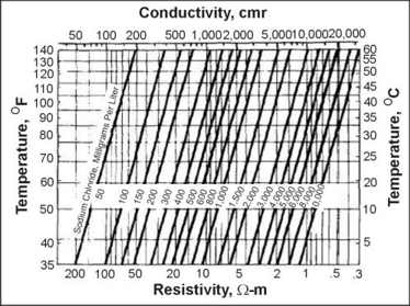
Figure 6. Electrically equivalent sodium chloride solution plotted as a function of conductivity or resistance and temperature.
Definition
By definition, resistivity is a function of the dimensions of the material being measured; therefore, it is an intrinsic property of that material. Resistivity is defined by the formula:
![]() (1)
(1)
where
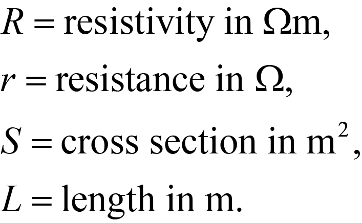
The principles of measuring resistivity are illustrated in figure 7. If 1 amp of current from a 10-V battery is passed through a 1-m3 block of material, and the drop in potential is 10 V, the resistivity of that material is 10 Wm. The current is passed between electrodes A and B, and the voltage drop is measured between potential electrodes M and N, which, in the example, are located 0.1 m apart-, so that 1 V is measured rather than 10 V. The current is maintained constant, so that the higher the resistivity between M and N, the greater the voltage drop will be. A commutated DC current is used to avoid polarization of the electrodes that would be caused by the use of direct current.
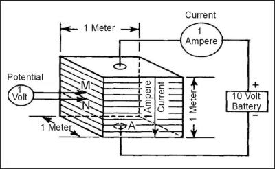
Figure 7. Principles of measuring resistivity in Ohm-meter. Example is 10 Ohm-meter.
Data Acquisition for Normal Resistivity Logs
AM spacing. For normal-resistivity logging, electrodes A and M are located in the well relatively close together, and electrodes B and N are distant from AM and from each other, as shown in figure 7. Electrode configuration may vary in equipment produced by different manufacturers. The electrode spacing, from which the normal curves derive their name, is the distance between A and M, and the depth reference is at the midpoint of this distance. The most common AM spacings are 40 and 162 cm (16 and 64 in); however, some loggers have other spacings available, such as 10, 20, 40 and 81 cm (4, 8, 16, and 32 in). The distance to the B electrode, which is usually on the cable, is approximately 15 m; it is separated from the AM pair by an insulated section of cable. The N electrode usually is located at the surface, but in some equipment, the locations of the B and N electrodes may be reversed. Constant current is maintained between an electrode at the bottom of the sonde and a remote-current electrode. The voltage for the long normal (162 cm (64 in)) and the short normal (40 cm (16 in)) is measured between a potential electrode for each, located on the sonde, and a remote potential electrode. The SP electrode is located between the short normal electrodes. The relative difference between the volumes of material investigated by the two normal systems also is illustrated in figure 8. The volume of investigation of the normal resistivity devices is considered to be a sphere, with a radius approximately twice the AM spacing. This volume changes as a function of the resistivity, so that its size and shape are changing as the well is being logged.
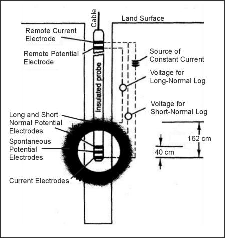
Figure 8. System used to make 40- and 162 cm (16- and 64-in) normal resistivity logs. Shaded areas indicate relative size volumes of investigation.
Depth of Invasion. Although the depth of invasion is a factor, short normal (40 cm (16 in or less)) devices are considered to investigate only the invaded zone, and long normal (162 cm (64 in)) devices are considered to investigate both the invaded zone and the zone where native formation water is found. These phenomena are illustrated in figure 360 . In this figure, the area between a 81 cm (32-in) curve on the left and a 10-cm (4-in) curve on the right is shaded. The longer spaced curve indicates a lower resistivity farther back in the aquifers than in the invaded zone near the borehole wall, which suggests that the formation water is relatively saline with respect to the borehole fluid.
Calibration. Normal-resistivity logging systems may be calibrated at the surface by placing fixed resistors between the electrodes. The formula used to calculate the resistor values to be substituted in the calibration network shown in figure 9 is given in Keys (1990).
Data Interpretation
Long normal response is affected significantly by bed thickness; this problem can make the logs quite difficult to interpret. The bed thickness effect is a function of electrode spacing, as illustrated in figure 10. The theoretical resistivity curve (solid line) and the actual log (dashed line) for a resistive bed, with a thickness six times the AM spacing, is shown in the top part of the figure. Resistivity of the limestone is assumed to be six times that of the shale, which is of infinite thickness. With a bed thickness six times AM, the recorded resistivity approaches, but does not reach, the true resistivity (Rt); the bed is logged as being one AM spacing thinner than it actually is. The actual logged curve is a rounded version of the theoretical curve, in part because of the effects of the borehole. The log response when the bed thickness is equal to or less than the AM spacing is illustrated in the lower half of figure 367. The curve reverses, and the high-resistivity bed actually appears to have a lower value than the surrounding material. The log does not indicate the correct bed thickness, and high-resistivity anomalies occur both above and below the limestone. Although increasing the spacing to achieve a greater volume of investigation would be desirable, bed-thickness effects would reduce the usefulness of the logs except in very thick lithologic units.
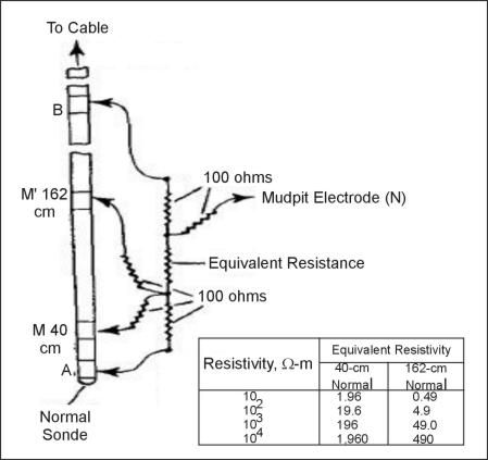
Figure 9. System for calibrating normal resistivity equipment.
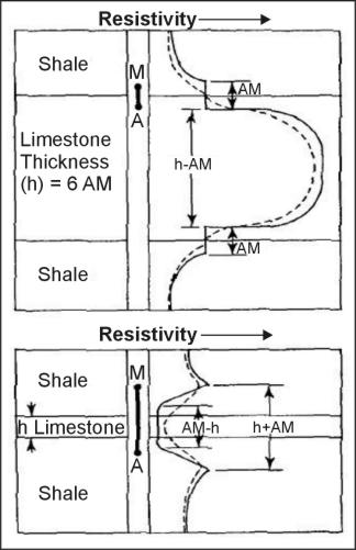
Figure 10. Relation of bed thickness to electrode spacing for normal devices at two thicknesses.
Applications
Water Quality. An important application of normal resistivity logs and other multi-electrode logs is to determine water quality. Normal logs measure apparent resistivity; if true resistivity is to be obtained from these logs, they must be corrected with the appropriate ts or departure curves. A summary of these techniques is found in "The Art of Ancient Log Analysis," compiled by the Society of Professional Well Log Analysts (1979). A practical method is based on establishing field-formation resistivity factors (F) for aquifers within a limited area, using electric logs and water analyses. After a consistent formation factor is established, the long normal curve, or any other resistivity log that provides a reasonably correct Rt can be used to calculate Rw from the relationship: F = Ro/Rw. Under these conditions, Ro, the resistivity of a rock 100% saturated with water, is assumed to approximate Rt, after the appropriate corrections have been made. Resistivities from logs can be converted to standard temperature using figure 5, and the factors listed in Keys (1990) can be used to convert water containing other ions to the electrically equivalent sodium chloride solution.
The formation resistivity factor (F) also defines the relation between porosity (Ø) and resistivity as follows: F = a/Øm = Ro/Rw, where m is the cementation exponent (Archie's formula). See Jorgensen (1989) for a more complete description of these relations. Using porosity derived from a neutron, gamma‑gamma, or acoustic velocity log, and Ro from a deep investigating resistivity log, one can determine the resistivity of the formation water in granular sediments. The relation between resistivity from normal logs and the concentration of dissolved solids in groundwater is only valid if the porosity and clay content are relatively uniform. The method does not apply to rocks with a high clay content or with randomly distributed solution openings or fractures. Surface conduction in clay also tends to reduce the resistivity measured. The resistivity logs in figure 3 were used to calculate the quality of the water in aquifers at the Kipling well site in Saskatchewan, Canada. The left trace of the two normal resistivity logs shown is the 81-cm (32-in) normal, which was used to calculate Rw for three of the shallower aquifers intersected. These aquifers are described as coarse, pebbly sand based on side-wall core samples. The 81-cm (32-in) normal was selected because many of the beds in this area are too thin for longer spacing. Wyllie (1963) describes a method for estimating F from the ratio Ri/Rm, where Ri is the resistivity of the invaded zone from a short normal log like the 10-cm (4-in), and Rm is the measured resistivity of the drilling mud. On the basis of the 10-cm (4-in) curve, F was estimated to be 2.5 for the upper aquifer and 1.8 for the lower two. The true resistivities for the three aquifers obtained from departure curves are 30, 20, and 17 Ώm at depths of 40, 76, and 90 m (130, 250, and 295 ft), respectively. A formation factor of 3.2 provided good agreement with water quality calculated from SP logs and from laboratory analyses. Using an F of 3.2, Rw was calculated to be 9.4, 6.2, and 5.3 Ώm at 4° C for the three aquifers. The drilling mud measured 13 Ώm at borehole temperature. The separation of the two normal curves and the SP log response substantiated the fact that the water in the aquifers was more saline than the drilling mud.
Lateral logs are made with four electrodes like the normal logs but with a different configuration of the electrodes. The potential electrodes M and N are located 0.8 m apart; the current electrode A is located 5.7 m above the center (O) of the MN spacing in the most common petroleum tool, and 1.8 m in tools used in groundwater. Lateral logs are designed to measure resistivity beyond the invaded zone, which is achieved by using a long electrode spacing. They have several limitations that have restricted their use in environmental and engineering applications. Best results are obtained when bed thickness is greater than twice AO, or more than 12 m for the standard spacing. Although correction ts are available, the logs are difficult to interpret. Anomalies are asymmetrical about a bed, and the amount of distortion is related to bed thickness and the effect of adjacent beds. For these reasons, the lateral log is not recommended for most engineering and environmental applications.
Focused resistivity systems were designed to measure the resistivity of thin beds or high-resistivity rocks in wells containing highly conductive fluids. A number of different types of focused resistivity systems are used commercially such as "guard" or "laterolog." Focused or guard logs can provide high resolution and great penetration under conditions where other resistivity systems may fail. Focused-resistivity devices use guard electrodes above and below the current electrode to force the current to flow out into the rocks surrounding the well. The depth of investigation is considered to be about three times the length of one guard, so a 1.8 m guard should investigate material as far as 5.5 m from the borehole. The sheetlike current pattern of the focused devices increases the resolution and decreases the effect of adjacent beds in comparison with the normal devices.
Microfocused devices include all the focusing and measuring electrodes on a small pad; they have a depth of investigation of only several centimeters. Because the geometric factor, which is related to the electrode spacing, is difficult to calculate for focused devices, calibration usually is carried out in a test well or pit where resistivities are known. When this is done, the voltage recorded can be calibrated directly in terms of resistivity. Zero resistivity can be checked when the entire electrode assembly is within a steel-cased interval of a well that is filled with water.
Correction for bed thickness (h) is only required if h is less than the length of M, which is 6 in. on some common tools. Resistivities on guard logs will approach Rt, and corrections usually will not be required if the following conditions are met: Rm/Rw < 5, Rt/Rm > 50, and invasion is shallow. If these conditions are not met, correction ts and empirical equations are available for obtaining Rt (Pirson, 1963).
A large number of microresistivity devices exist, but all employ short electrode spacing so that they have a shallow depth of investigation. They can be divided into two general groups: focused and non-focused. Both groups employ pads or some kind of contact electrodes to reduce the effect of the borehole fluid. Non-focused sondes are designed mainly to determine the presence or absence of mud cake, but they also can provide very high-resolution lithologic detail. Names used for these logs include microlog, minilog, contact log, and micro-survey log. Focused microresistivity devices also use small electrodes mounted on a rubber-covered pad forced to contact the wall of the hole hydraulically or with heavy spring pressure. The electrodes are a series of concentric rings less than 2.5 cm apart that function in a manner analogous to a laterolog system. The radius of investigation is from 76 to 127 mm, which provides excellent lithologic detail beyond the mudcake, but probably is still within the invaded zone.
The dipmeter includes a variety of wall-contact microresistivity devices that are widely used in oil exploration to provide data on the strike and dip of bedding planes. The most advanced dipmeters employ four pads located 90° apart, oriented with respect to magnetic north by a magnetometer in the sonde. Older dipmeters used three pads 120° apart. The modern dipmeter provides a large amount of information from a complex tool, so it is an expensive log to run. Furthermore, because of the amount and complexity of the data, the maximum benefit is derived from computer analysis and plotting of the results. Interpretation is based on the correlation of resistivity anomalies detected by the individual arms, and the calculation of the true depth at which those anomalies occur. The log from a four-arm tool has four resistivity curves and two caliper traces, which are recorded between opposite arms, so that the ellipticity of the hole can be determined. The Formation Microscanner is related to the dipmeter. It uses arrays of small electrodes to provide oriented conductance images of segments of the borehole wall scanned by the pads. These images are similar to an acoustic televiewer log, but they do not include the entire borehole wall. The microscanner may be preferable in heavy muds or deviated holes.
Although strike and dip can be determined from the analog record at the well using a stereo net, complete analysis is only possible with a computer. A computer program can make all necessary orientation and depth corrections and search for correlation between curves with a selected search interval. Computer output usually consists of a graphic plot and a listing of results. The graphic plot displays the depth, true dip angle, and direction of dip by means of a symbol called a "tadpole" or an arrow. The angle and direction of the tool also is displayed. Linear polar plots and cylindrical plots of the data also are available. A printout that lists all the interpreted data points, as well as the quality of the correlation between curves, also is provided.
The dipmeter is a good source of information on the location and orientation of primary sedimentary structures over a wide variety of hole conditions. The acoustic televiewer can provide similar information under the proper conditions. The dipmeter also has been advertised widely as a fracture finder; however, it has some of the same limitations as the single-point resistance log when used for this purpose. Computer programs used to derive fracture locations and orientations from dipmeter logs are not as successful as those designed for bedding. Fractures usually are more irregular, with many intersections, and may have a wider range of dip angles within a short depth interval. The acoustic televiewer provides more accurate fracture information under most conditions.
Basic Concept
Induction logging devices originally were designed to make resistivity measurements in oil-based drilling mud, where no conductive medium occurred between the tool and the formation. The basic induction logging system is shown in figure 11. A simple version of an induction probe contains two coils: one for transmitting an AC current, typically 20 to 40 kHz, into the surrounding rocks, and a second for receiving the returning signal. The transmitted AC generates a time-varying primary magnetic field, which induces a flow of eddy currents in conductive rocks penetrated by the drill hole. These eddy currents set up secondary magnetic fields, which induce a voltage in the receiving coil. That signal is amplified and converted to DC before being transmitted up the cable. Magnitude of the received current is proportional to the electrical conductivity of the rocks. Induction logs measure conductivity, which is the reciprocal of resistivity. Additional coils usually are included to focus the current in a manner similar to that used in guard systems. Induction devices provide resistivity measurements regardless of whether the fluid in the well is air, mud, or water, and excellent results are obtained through plastic casing. The measurement of conductivity usually is inverted to provide curves of both resistivity and conductivity. The unit of measurement for conductivity is usually milliSiemens per meter (mS/m), but millimhos per meter and micromhos per centimeter are also used. One mS/m is equal to 1,000 Ώm. Calibration is checked by suspending the sonde in air, where the humidity is low, in order to obtain a zero conductivity. A copper hoop is suspended around the sonde while it is in the air to simulate known resistivity values. The volume of investigation is a function of coil spacing, which varies among the sondes provided by different service companies. For most tools, the diameter of material investigated is 1.0 to 1.5 m; for some tools, the signal produced by material closer to the probe is minimized. Figure 12 shows the relative response of a small-diameter, high-frequency induction tool as a function of distance from the borehole axis. These smaller diameter tools, used for monitoring in the environmental field, can measure resistivities up to 1,000 Ώm.
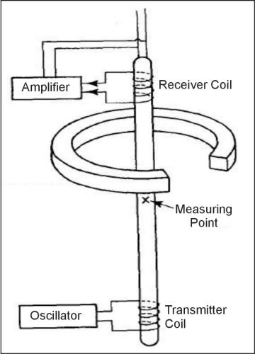
Figure 11. System used to make induction logs.
Data Interpretation
Induction logs are becoming widely used on environmental projects for monitoring saline contaminant plumes by logging small-diameter, PVC- or fiberglass-cased wells. They also provide high-resolution information on lithology through casing and are excellent for this purpose when combined with gamma logs. The response curve in figure 12 is for a tool that can be used in 5-cm diam (2-in) casing. Figure 13 is a comparison of induction resistivity logs in an open and cased well with a 40-cm (16-in) normal resistivity log. The open hole was 23 cm (9 in) and drilled with a mud rotary system. The well was completed to a depth of 56 m with 20-cm (4-in) Schedule 80 PVC casing and neat cement, bentonite seal, and gravel pack. Even in such a large- diameter well with varying completion materials, the differences in resistivity are not significant.
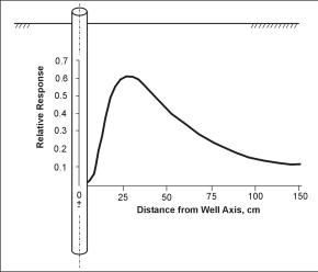
Figure 369. Relative response of an induction probe with radial distance from borehole axis (copyright permission granted by Geonics Ltd.).
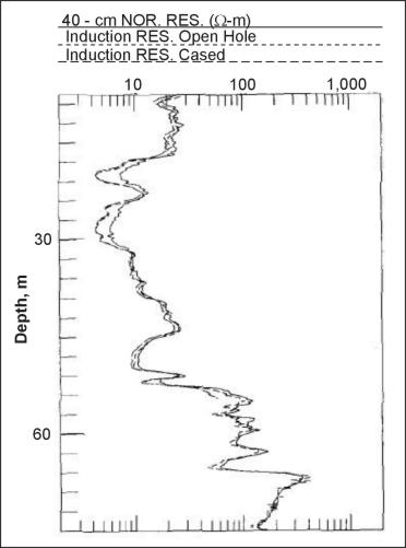
Figure 13. Comparision of open hole induction log with normal log and induction log made after casing was installed. (copyright permission granted by Colog, Inc.)
The pages found under Surface Methods and Borehole Methods are substantially based on a report produced by the United States Department of Transportation:
Wightman, W. E., Jalinoos, F., Sirles, P., and Hanna, K. (2003). "Application of Geophysical Methods to Highway Related Problems." Federal Highway Administration, Central Federal Lands Highway Division, Lakewood, CO, Publication No. FHWA-IF-04-021, September 2003. http://www.cflhd.gov/resources/agm/