Environmental Geophysics
Inversion
Introduction
Geophysics is a tool to explore the subsurface using a limited set of remote measurements. Different geophysical methods study different properties of the earth. For example, electrical and electromagnetic methods study the resistivity and seismic methods measure the density and elastic properties. Geophysics is a natural tool to complement standard geochemical or hydrogeological in situ sampling in wells, in providing spatio-temporal infomation that cannot be reached by direct sampling. Inversion is a post-processing step, where geophysical parameters can be transformed to geologic data, existence of oil, minerals, and water content, for instance.
Theory
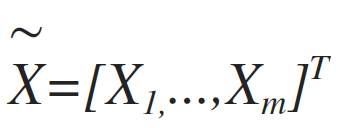
In usual data processing, a geophysicist is seeking the estimation of those parameters, which usually are denoted as X - model, by using a limited set or measurements denoted as d - data. These parameters of the inversion model are usually found in a (either 1D, 2D or 3D) gird and can be expresses as a vector, i.e.
 (1)
(1)
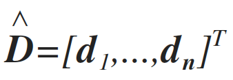
Where Xi is i.e the resistivity or seismic arrival times value on grid node ith. m is the total number of parameters to be estimated. The measurements d, are also expresses as a vector of i.e voltages or arrival times, i.e
 (2)
(2)
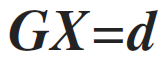
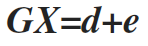
Where n is the number of measurements collected. In most cases, the connection between the model and the data can be written as a set of equations that, with the use of linear algebra, is expressed as:
 (3)
(3)
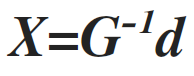
Where G is called the forward operator. This forward operator describes our understating for the physics of the problem, i.e. if the resistivity structure of earth (X) is known, then the application of the operator G will give us the potentials (d) in the gridded space; if the velocities of the propagation of p-waves are known (m), then the operator G gives the arrival time to the geophones (d). Usually calculation of the forward operator evolves the solution of a partial differential equation (PDE). Estimation of the model X, given the data d is part of the inversion process. This can be expressed as
 (4)
(4)
Where G-1 is the inverse operator.
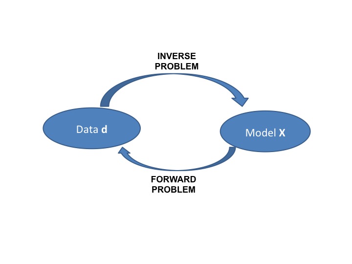
Figure 1. The forward and inverse problem.
Most of the times the inverse operator cannot be applied due to the following reasons.
This is the reason why inverse problems are so challenging. Another major problem to the inverse problem is the existence of noise. Noise is hidden in the data (random measurement errors) and due to the simplification of the forward operator (i.e. discretization of continuous function, and numerical solution that is an approximation of the "true" physics).
Taken into account all of the above we can re-write the inversion problem as
 (5)
(5)
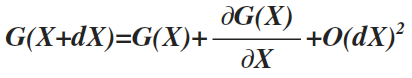
Where e is the random noise. Therefore the inverse problem is transform into an optimization problem, where we seek a solution (a model) that minimizes that error e. There are several approaches on this optimization problem that cannot be covered on an introductory text. Briefly we mention that they can be summarized into two large categories, the gradient based and the stochastic based schemes. It is important to notice at this point, that some geophysical are non-linear and therefore we can go from data to model in one step. In those cases, we can linearize the problems, by taking the Taylor expansion
 (6)
(6)
Where O(dX)2 are higher order terms, that we can neglect. The above expression implies that although there is non linearity from the model to data, there is linearity from the changes of the models and the changes of the data. Thus, non linear problems can be solved iterativly, starting from an initial model, iteratively update it until the misfit is small enough. This can be express with the following flowchart
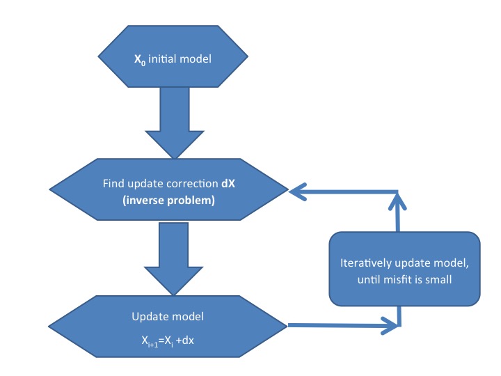
Figure 2. The inverse model flowchart.
Gradient Based Algorithms
There are many different proposed algorithms on the solution of the inverse problem (linear or non-linear), where most of them are based on the minimization of some norm (1st norm, 2nd norm etc) of the error with respect the norm of the model. We will briefly describe the most popular gradient based, the least squares smoothness constrained inversion, which is an l2-norm. The main principles of this approach can be summarized on the following expression, if in doubt smooth. This approach searches from all the possible models that fits the data, choose one that may not for perfectly the data but it is smooth. The definition of smooth comes from geological observations: geology is appearing (most likely) in a layered sense, and therefore not extremely big changes are observed in nearby spatial points. Therefore the optimization problem, is expressed as a minimization of the following objective function
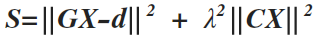 (7)
(7)
where λ denotes the tradeoff parameter that controls the model regularization and C is the second derivative of the model. The first term of the objective functions, ensures the convergence of the recovered model with respect to the observed data. The second part of the objection function, is introduced to stabilize the inversion algorithm, and produce smooth models (Constable et al., 1987). The solution to this objective function is found either with an iterative Occam's update Equation
 (8)
(8)
where I denotes the iteration number, dx is the update model and J is the Jacobian or sensitivity matrix. Consider a 2D area discretization, with 3x3 parameters (total 9 parameters). Then smoothness matrix C, is a 9x9 matrix with the following form (each color represents a corresponding value).
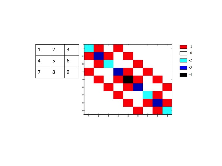
Figure 3. A second derivative of a smoothness matrix, for a 3x3 2D discretization.
The Lagrange parameter λ, controls the effect of smoothness on the inversion. Small values makes the inversion unstable, large values smooth the model too much. So the optimum value of this multiplies is crucial: and it’s a continuously active topic. Generally, the search of an optimum value should start with a full analysis of the inverse equations. Such an analysis can be performed by using the Singular Value Decomposition (SVD) of the inverse matrix. If G is an mxn matrix, then the SVD analysis og this matrix gives
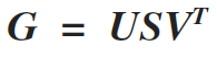 (9)
(9)
Where U is an m x m real or complex unitary matrix, S is an m x n rectangular diagonal matrix with nonnegative real numbers on the diagonal, and VT (the conjugate transpose of V) is an n x n real or complex unitary matrix. The diagonal entries Si,i of S are known as the singular values of M,. The m columns of U and the n columns of V are called the left singular vectors and right singular vectors of M, respectively. Since G shows an rank deficient problem, some of the values of Si,i of S are very small (or even zero), making the inverse operator unstable. Several approach can address this problem, which we will not discuss here.
Some more sophisticated approaches are based on the trial of different values of the Lagrange multiplier, and plot the corresponding values of ∥X∥ and ∥GX-d∥. This plot shows a characteristic l-shape curve, where it's corner is the optimum Lagrange value (as shown by many authros). This of course implies that of each Lagrange test, we need to solve the forward problem, something that it is very consuming.
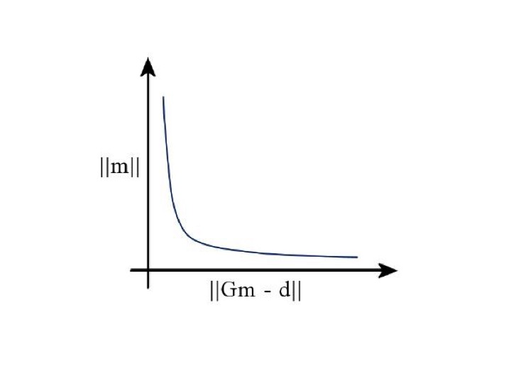
Figure 4. The I-curve as a tool of finding the optimum Lagrange value.
Among different techniques proposed to find the tradeoff parameter, in this work two methods are used. Using an empirical value for the space domain tradeoff parameter, and starting with a relatively large value (0.15 is suggested by default), is decreased with the number of iterations. The space-domain tradeoff parameter is expressed as a diagonal matrix Λ because the active constraint balancing (ACB) (Yi et al., 2003) is adapted for the space-domain regularization. Briefly, this technique assigns different tradeoff values depending on the resolution matrix R
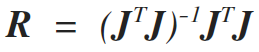 (10)
(10)
Values that are well resolved are assigned a small tradeoff parameter. Conversely, parameters that are poorly resolved are associated with large values of the tradeoff parameter. Although the parameter resolution matrix shows the resolution of the parameters, it cannot give a quantitative measure of the goodness of resolution for the intermediate range between perfect and very poor. To quantify the resolving power, we use the Backus-Gilbert spread function (Menke, 1984), which evaluates the spatial distribution of the row vectors of the parameter resolution matrix. A large value of spread function for a certain parameter means that the resolution of that parameter is degenerated, or vice versa. This spread function is calculated for the ith parameter as,
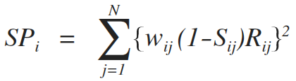 (11)
(11)
where N is the number of parameters, and wij is a weighting factor, computed from the spatial distance between the two parameters i and j . Here, Sij is a matrix used to take into account the constraint or regularization in the inversion (i.e., the effect of the damping or smoothing operator). Sij is unity when Cij is nonzero, and is zero otherwise. This spread function can be used as a tool for the resolution or sensitivity analysis of the inverse problem. An example of the effect of this approach follows on the next figure, where borehole to surface measurements are considered. Close to areas where we have receivers (and therefore a lot of information) the algorithm suggest small Lagrange values and vice versa.
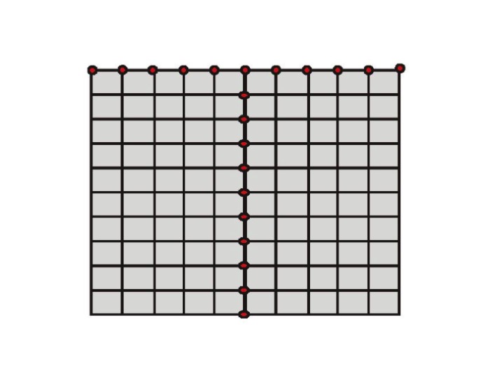
Figure 5. A borehole to surface measurement configuration array. Red dots indicate the receiver location.
The inversion results
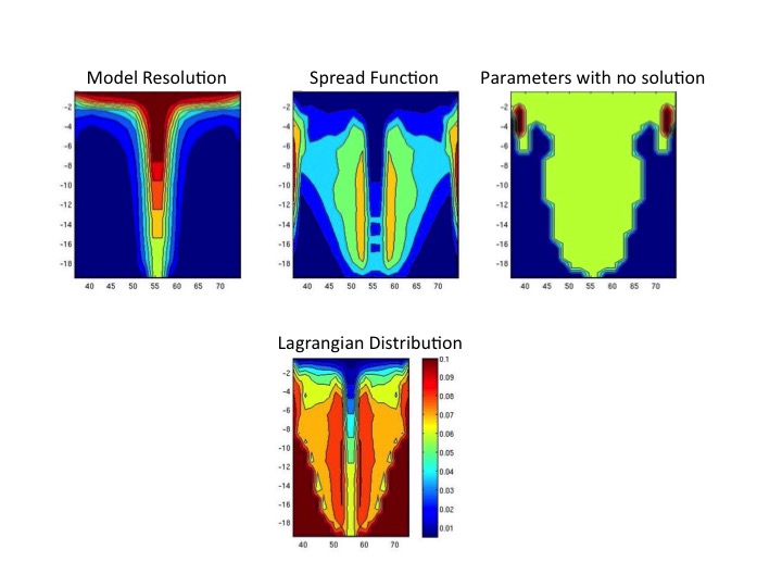
Figure 6. Lagrange distribution based on the resolution matrix. The spread function is calculated based on the resolutions and is responsible for the distribution of the final Lagrange values. As it is expected, small values are observed close to the receivers.
Notes for further reading
Inversion theory is a constant evolving theory. There are many text books that cover this topic, which we will not list them her. Authors found very useful and easy to understand "Parameter Estimation and Inverse Problem, Aster R.C., Borchers B., Thurber C. H. Academic Press; 1 edition (January 11, 2005)" A classical text book for the stochastic approach is "Inverse theory and methods for model parameter estimation. Tarantola A. SIAM: Society for Industrial and Applied Mathematics; 1 edition (December 20, 2004)
Special thanks to Marios Karaoulis, who contributed to this Inversion page.