Basic Concept

Lateral density changes in the subsurface cause a change in the force of gravity at the surface.  The intensity of the force of gravity due to a buried mass difference (concentration or void) is superimposed on the larger force of gravity due to the total mass of the earth.  Thus, two components of gravity forces are measured at the Earth's surface: first, a general and relatively uniform component due to the total earth, and second, a component of much smaller size that varies due to lateral density changes (the gravity anomaly).  By very precise measurement of gravity and by careful correction for variations in the larger component due to the whole Earth, a gravity survey can sometimes detect natural or man-made voids, variations in the depth to bedrock, and geologic structures of engineering interest. 

For engineering and environmental applications, the scale of the problem is generally small (targets are often from 1 to 10 m in size).  Therefore, conventional gravity measurements, such as those made in petroleum exploration, are inadequate.  Station spacings are typically in the range of 1 to 10 m.  Even a new name, microgravity, was invented to describe the work.  Microgravity requires preserving all of the precision possible in the measurements and analysis so that small objects can be detected.

The interpretation of a gravity survey is limited by ambiguity and the assumption of homogeneity.  A distribution of small masses at a shallow depth can produce the same effect as a large mass at depth.  External control of the density contrast or the specific geometry is required to resolve ambiguity questions.  This external control may be in the form of geologic plausibility, drill-hole information, or measured densities.

The first question to ask when considering a gravity survey is for the current subsurface model, can the resultant gravity anomaly be detected?  To answer this question the information required are the probable geometry of the anomalous region, its depth of burial, and its density contrast.  A general rule of thumb is that a body must be almost as big as it is deep.  To explore this question, figure 1 was prepared.  The body under consideration is a sphere.  The vertical axis is normalized to the attraction of a sphere whose center is at a depth equal to its diameter.  For illustration, the plotted values give the actual gravity values for a sphere 10 m in diameter with a 1,000 kg/m³ (1.0 g/cc) density contrast.  The horizontal axis is the ratio of depth to diameter.  The rapid decrease in value with depth of burial is evident.  At a ratio of depth to diameter greater than 2.0, the example sphere falls below the practical noise level for most surveys as will be discussed below.

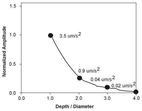
Figure 1.  Normalized peak vertical attraction versus depth to diameter for a spherical body.  Values are for a 10-m sphere with a 1.0 g/cc density contrast.

A second rule of thumb is that unless you are very close to the body, its exact shape is not important.  Thus, a rectangular-shaped horizontal tunnel sometimes can be modeled by a horizontal circular cylinder, and a horizontal cylinder sometimes can be modeled by a horizontal line source.  Odd-shaped volumes can be modeled by disks, and where close to the surface, even infinite or semi-infinite slabs.

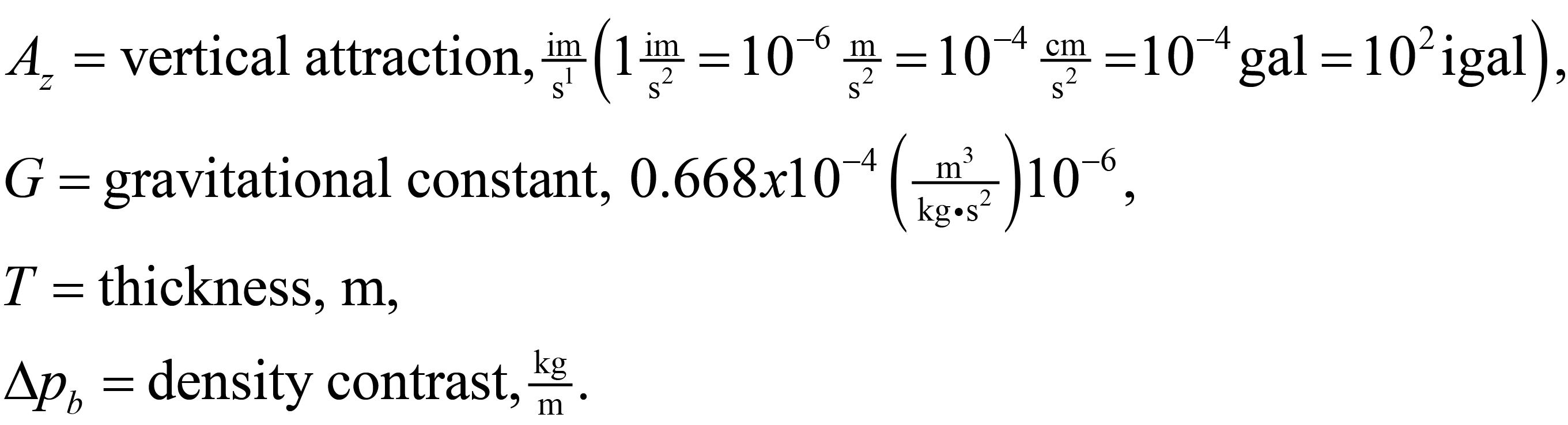
Among the many useful nomograms that are available, Figure 2, shown below (which is adapted from Arzi, 1975) is very practical.  The gravity anomaly is linear with density contrast so other density contrasts can be evaluated by scaling the given curves.  For cylinders of finite length, very little correction is needed unless the cylinder length is less than four times its width.  Nettleton (1971) gives the correction formula for finite length of cylinders.  Another useful simple formula is the one for an infinite slab.  This formula is:

                                                                                               (1)

where

As an example, consider a 1-m-thick sheet with a density contrast with its surroundings twice that of water. From equation 1, the calculation would be A_z = 2 π (0.668x10 -4 )(1.0)(2,000) m m/s² = 0.84 m m/s² .

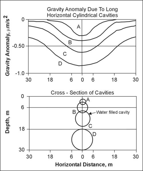
Figure 2. Gravity anomalies for long horizontal cylindrical cavities as a function of depth, size, and distance from peak.

A surprising result from potential theory is that there is no distance term in this formula. The intuitive objections can be quelled by focusing on the fact that the slab is infinite in all directions. The usefulness of this formula increases if one recognizes that the attraction of a semi-infinite slab is given by one-half of the above formula at the edge of the slab. Thus, near the edge of a fault or slab-like body, the anomaly will change from zero far away from the body to (2πGtΔp_b) at a point over the body and far away from the edge (above the edge the value is 2πGtΔp_b ). This simple formula can be used to quickly estimate the maximum response from a slab-type anomaly. If the maximum due to the infinite sheet is not detectable, then complicated calculations with finite bodies are not justified. Nettleton (1971) is a good source of formulas that can be used to approximate actual mass distributions.

Items that should not be overlooked in estimating the probable density contrast are:

•  Variability (1,000 to 3,500 kg/m³ ) of the density of rocks and soils.

•  Possibility of fractures and weathering in rocks.

•  Probability of water filling in voids.

Each of these items should be individually considered before a density contrast is set. The effects of upward-propagating fractures, which can move a mass deficiency nearer the surface, and the presence or absence of air pockets usually cannot be evaluated if one is after subsurface mass deficiencies. However, these effects will increase the amplitude of the anomaly, sometimes by a factor of two or more.

Data Acquisition

Usually more important in a feasibility study than the anomaly evaluation is the estimation of the noise sources expected. This section will discuss the larger contributions to noise and evaluate each.

Modern gravimeters have a least-significant scale reading of 0.01 µm/s². However, repeated readings including moving the meter, releveling, and unclamping the beam several times indicate an irreducible meter reading error of about 0.05 µm/s². New electronically augmented versions of these gravimeters consistently repeat to 0.02 to 0.03 µm/s². Some surveys may do slightly better, but one should be prepared to do worse. Factors that may significantly increase this type of error are soft footing for the gravimeter plate (surveys have been done on snow), wind, and ground movement (trucks, etc.) in the frequency range of the gravimeter. Again, the special versions of these gravimeters that filter the data appropriately can compensate for some of these effects. A pessimist, with all of the above factors in action, may allow 0.08 to 0.1 µm/s² for reading error.

Gravity measurements, even at a single location, change with time due to Earth tides, meter drift, and tares. These time variations can be dealt with by good field procedure. The Earth tide may cause changes of 2.4 µm/s² in the worst case, but it has period of about 12.5 hours; it is well approximated as a straight line over intervals of 1 to 2 hours, or it can be calculated and removed. Drift is also well eliminated by linear correction. Detection of tares and blunders (human inattention) is also a matter of good field technique and repeated readings. One might ascribe 10 to 20 nm/s² to these error sources.

Up to 50% of the work in a microgravity survey is consumed by the survey. For the very precise work described above, relative elevations for all stations need to be established to +/-1 to 2 cm. A firmly fixed stake or mark should be used to allow the gravity meter reader to recover the exact elevation. Position in plan is less critical, but relative position to 50-100 cm or 10 percent of the station spacing (whichever is smaller) is usually sufficient. Satellite surveying, GPS, can achieve the required accuracy, especially the vertical accuracy, only with the best equipment under ideal conditions.

High station densities are often required. It is not unusual for intervals of 1-3 m to be required to map anomalous masses whose maximum dimension is 10 m. Because the number of stations in a grid goes up as the square of the number of stations on one side, profiles are often used where the attitude of the longest dimension of the sought body can be established before the survey begins.

After elevation and position surveying, actual measurement of the gravity readings is often accomplished by one person in areas where solo work is allowed. Because of short-term variations in gravimeter readings caused by less than perfect elasticity of the moving parts of the suspension, by uncompensated environmental effects, and by the human operator, it is necessary to improve the precision of the station readings by repetition. The most commonly used survey technique is to choose one of the stations as a base and to reoccupy that base periodically throughout the working day. The observed base station gravity readings are then plotted versus time, and a line is fitted to them to provide time rates of drift for the correction of the remainder of the observations. Typically, eight to ten measurements can be made between base station occupations; the time between base readings should be on the order of 1-2 hr. Where higher precision is required, each station must be reoccupied at least once during the survey.

If even higher precision is desired or if instrumental drift is large in comparison with the expected gravity anomaly, then a leapfrogging of stations can be used. For example, if the stations are in an order given by a,b,c,d,e,f,. then the station occupations might be in the sequence ab, abc, abcd, bcde, cdef, defg, etc. In this way, each station would be occupied four times. Numerical adjustments, such as least squares minimization of deviations, may be applied to reoccupation data sets. This procedure allows data quality to be monitored and controlled and distributes any systematic errors throughout the grid.

If base reoccupations are done approximately every hour, known errors such as the earth tide are well approximated by the removal of a drift correction that is linear with time. Even if the theoretical earth tide is calculated and removed, any residual effects are removed along with instrumental drift by frequent base station reoccupation.

Data Processing

Four main corrections are made to gravity data:

•  International Gravity formula accounts for the variation of gravity with latitude.

•  The Free Air correction accounts for the change of gravity for the distance of the station above a datum (sea level) and the station at an elevation Δh.

•  The Bouguer correction accounts for the attraction of the rock material between a datum level and the station at an elevation Δh.

•  Topographic corrections account for all the materialshigher than the gravity stations and removes the effect of the material needed to fill in any hollow below the station.

Details of the free air, Bouguer slab, and terrain corrections will not be expressed here (see Blizkovsky, 1979), but the formula will be given.

The International Gravity formula or variation of gravity with latitude is given by:

 

           (2)

 

                                                                  

where

g = acceleration of gravity in m/s² ,

Φ = latitude in degrees.

Calculations show that if the stations at which gravity are collected are located with less than 0.5 to 1.0 m of error, the error in the latitude variation is negligible. In fact, for surveys of less than 100 m north to south, this variation is often considered part of the regional and removed in the interpretation step. Where larger surveys are considered, the above formula gives the appropriate correction.

The free-air and the Bouguer slab are corrected to a datum by the following formula (the datum is an arbitrary plane of constant elevation to which all the measurements are referenced):

                                       (3)

            where                      

G_s = simple Bouguer corrected gravity value measured in m m/s² ,

G_OBS = observed gravity value in m m/s² ,

Δp b = near-surface density of the rock in kg/m³ ,

Δh = elevation difference between the station and datum in meters.

If these formulas were analyzed, see that the elevation correction is about 20 nm/s² per cm. It is impractical in the field to require better than @ 1 to 1.5 cm leveling across a large site, so 30 to 40 nm/s² of error is possible due to uncertainty in the relative height of the stations and the meter at each station.

The formula for free air and Bouguer corrections contains a surface density value in the formulas. If this value is uncertain by ±10 percent, its multiplication times Δh can lead to error. Obviously, the size of the error depends on Δh, the amount of altitude change necessary to bring all stations to a common level. The size of the Δh for each station is dependent on surface topography. For a topographic variation of 1 m (a very flat site!), the 10% error in the near-surface density corresponds to ±60 nm/s². For a ±10-m site, the error is ±0.6 m m/s². All of these estimates are based on a mistaken estimate of the near-surface-density, not the point-to-point variability in density, which also may add to the error term.

The terrain effect (basically due to undulations in the surface near the station) has two components of error. One error is based on the estimate of the amount of material present above and absent below an assumed flat surface through the station. This estimate must be made quite accurately near the station; farther away some approximation is possible. In addition to the creation of the geometric model, a density estimate is also necessary for terrain correction. The general size of the terrain corrections for stations on a near flat (±3-m) site, the size of tens of acres might be 1 m m/s². A 10% error in the density and the terrain model might produce ±0.1  m m/s² of error. This estimate does not include terrain density variations. Even if known, such variations are difficult to apply as corrections.

To summarize, a site unsuited for microgravity work (which contains variable surface topography and variable near-surface densities) might produce 0.25 to 0.86  m m/s² of difficult-to-reduce error.

Rock Properties . Values for the density of shallow materials are determined from laboratory tests of boring and bag samples. Density estimates may also be obtained from geophysical well logging. Table 1 lists the densities of representative rocks. Densities of a specific rock type on a specific site will not have more than a few percent variability as a rule (vuggy limestones being one exception). However, unconsolidated materials such as alluvium and stream channel materials may have significant variation in density.

Once the basic latitude, free-air, Bouguer and terrain corrections are made, an important step in the analysis remains. This step, called regional-residual separation, is one of the most critical. In most surveys, and in particular those applications in which very small anomalies are of greatest interest, there are gravity anomaly trends of many sizes. The larger sized anomalies will tend to behave as regional variations, and the desired smaller magnitude local anomalies will be superimposed on them. A simple method of separating residual anomalies from microregional variations is simply to visually smooth contour lines or profiles and subtract this smoother representation from the reduced data. The remainder will be a residual anomaly representation. However, this method can sometimes produce misleading or erroneous results.

Several automatic versions of this smoothing procedure are available including polynomial surface fitting and band-pass filtering. The process requires considerable judgment and, whichever method is used, should be applied by an experienced interpreter.

Note that certain unavoidable errors in the reduction steps may be removed by this process. Any error that is slowly varying over the entire site, such a distant terrain or erroneous density estimates, may be partially compensated by this step. The objective is to isolate the anomalies of interest. Small wavelength (about 10 m) anomalies may be riding on equally anomalous measurements with wavelengths of 100 or 1,000 m. The scale of the problem guides the regional-residual separation.

Data Interpretation 

Software packages for the interpretation of gravity data are plentiful and powerful.  The ease of use as determined by the user interface may be the most important part of any package.  The usual inputs are the residual gravity values along a profile or traverse.  The traverse may be selected from a grid of values along an orientation perpendicular to the strike of the suspected anomalous body.  Some of the programs allow one additional chance for residual isolation.  The interpreter then constructs a subsurface polygonal-shaped model and assigns a density contrast to it.  When the trial body has been drawn, the computer calculates the gravity effect of the trial body and shows a graphical display of the observed data, the calculated data due to the trial body, and often the difference.  The geophysicist can then begin varying parameters in order to bring the calculated and observed values closer together. 
 

Table 1.  Density approximations for representative rock types.

Parameters usually available for variation are the vertices of the polygon, the length of the body perpendicular to the traverse, and the density contrast.  Most programs also allow multiple bodies.

Because recalculation is done quickly (many programs work instantaneously as far as humans are concerned), the interpreter can rapidly vary the parameters until an acceptable fit is achieved.  Additionally, the effects of density variations can be explored and the impact of ambiguity evaluated.

Case Study 

Two examples were prepared to illustrate the practical results of the above theoretical evaluations.  The geologic section modeled is a coal bed of density 2,000 kg/m³ and 2 m thickness.  This bed, 9 m below the surface, is surrounded by country rock of density 2,200 kg/m³.  A water-filled cutout 25 m long and an air-filled cutout 12 m long are present.  The cutouts are assumed infinite perpendicular to the cross-section shown at the bottom of figure 246.  The top of figure 3 illustrates the theoretical gravity curve over this geologic section.  The middle curve is a simulation of a measured field curve.  Twenty-two microgals of random noise have been added to the values from the top curve as an illustration of the effect of various error sources.  The anomalies are visible, but quantitative separation from the noise might be difficult.

 

Figure 3.  Geologic model (bottom) including water- and air-filled voids; theoretical gravity anomaly (top) due to model; and possible observed gravity (middle), if 22 microgals (0.22 μm/s² ) of noise is present.  Depth of layer is 10 m.

Figure 4 is the same geologic section, but the depth of the coal workings is 31 m.  The anomalies are far more subtle (note scale change) and, when the noise is added, the anomalies disappear. For the two cases given, figure 4 represents a clearly marginal case.  Several points need to be discussed.  The noise added represents a compromise value.  In a hilly eastern coalfield on a rainy day, 0.22 μm/s² of error is optimistic.  On a paved parking lot or level tank bottom, the same error estimate is too high.  Note that the example uses random noise, whereas the errors discussed above (soil thickness variations, etc.) will be correlated over short distances. 

Another point is the idea of fracture migration or halo effect.  Some subsidence usually occurs over voids, or, in the natural case, the rock near caves may be reduced in density (Butler 1984).  The closer to the gravimeter these effects occur, the more likely is detection.

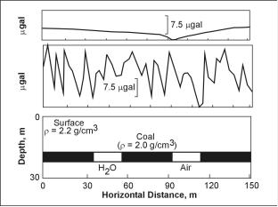
Figure 4.  Geologic model (bottom) including water and air filled voids, theoretical gravity anomaly (top) due to model; and possible observed gravity (middle), if 22 microgals of noise is present.  Depth of layer is 31 m.

Figure 5 illustrates a high precision survey over a proposed reservoir site.  The large size of the fault and its proximity to the surface made the anomaly large enough to be detected without the more rigorous approach of microgravity.  The area to the east is shown to be free of faulting (at least at the scale of tens of meters of throw) and potentially suitable as a reservoir site.

In addition to anomaly evaluation, the source and size of the irreducible field errors must be considered.  Under the proper conditions of large enough anomalies, good surface conditions, and some knowledge of densities, microgravity can be an effective tool for engineering investigations.  Figure 6 takes the one dimensional concepts discussed above, and extrapolates them to a two dimensional data set, providing a regional distribution of the gravity measurements. One common approach is to acquire regional data and extract transects for 1D modeling.

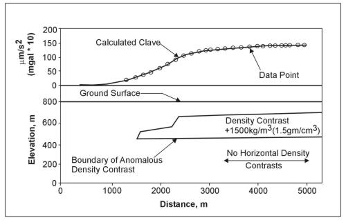
Figure 5.  Gravity traverse and interpreted model

 

 

 

 

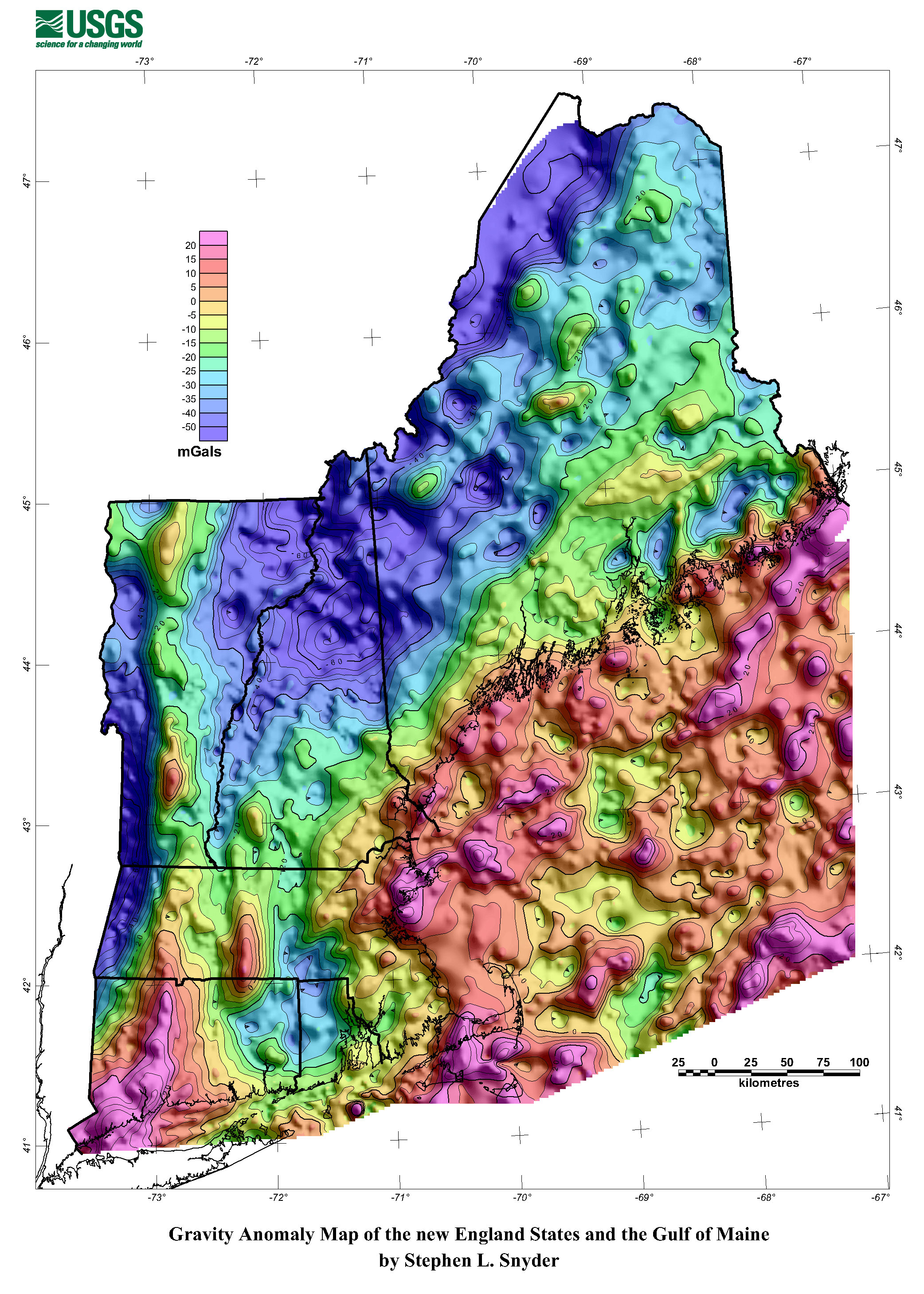
Figure 6. Gravity anomaly of the New England States and the Gulf of Maine (http://pubs.usgs.gov/of/2004/1258/HTML/NE_grav_small_map.htm).

 

 

The pages found under Surface Methods and Borehole Methods are substantially based on a report produced by the United States Department of Transportation:

Wightman, W. E., Jalinoos, F., Sirles, P., and Hanna, K. (2003). "Application of Geophysical Methods to Highway Related Problems." Federal Highway Administration, Central Federal Lands Highway Division, Lakewood, CO, Publication No. FHWA-IF-04-021, September 2003. http://www.cflhd.gov/resources/agm/

Top of Page

http://www.clu-in.org/characterization/technologies/geophysics/pages/reference/methods/Surface_Geophysical_Methods/Potentia_Field_Methods/Gravity_Methods.cfm
Last updated on Friday, September 16, 2016
Disclaimer, Privacy, and Security Notice | Site Map | About CLU-IN | Contact Us
Sponsored by the U.S. EPA Office of Superfund Remediation and Technology Innovation