XRF instruments are field-portable or handheld devices for simultaneously measuring metals and other elements in various media.

Top of Page

Energy dispersive X-ray fluorescence (EDXRF) is a method of detecting metals and other elements, such as arsenic, selenium, bromine, and iodine, in soil and sediment. Some of the primary elements of environmental concern that EDXRF can identify are arsenic, barium, cadmium, chromium, copper, lead, mercury, selenium, silver, and zinc. Most instruments can be made to detect any element between atomic weight 19 (potassium) and 92 (uranium). Some will detect 11 (sodium) through 94 (plutonium), with lighter elements (atomic weight 11 to 18) 11 to 18 having higher detection limits than heavier elements. The handheld or field-portable (FPXRF) units use techniques that have been developed for analysis of numerous environmental contaminants in soil and sediment. They provide data in the field that can be used to identify and characterize contaminated sites and guide remedial work, among other applications. An eight-part August 2008 XRF Web seminar is available with supporting materials in the CLU-IN Seminar Archive. The course manual is available for a January 2010 8-hour classroom course on XRF applications, XRF-specific QA/QC and data use.

FPXRF analyzers also have found use in identifying surfaces coated with paints that were cut with polychlorinated biphenyls (PCBs). A high chlorine content, which is generally not found in paints, can be indicative of PCBs. The use of PCBs in paints occurred in the 1950s through 1970s until they were banned. Older military activities, and Department of Energy facilities, utilities, and other industrial sites may have this problem.

Air particulate matter can be collected on a filter using a low- or high-volume sampler. The filter can then be removed and the elemental content measured by XRF. Appendix Q in 40 CFR 50 contains a (June 1999) method of how this is done for lead PM10 filter analysis.

FPXRF analyzers also can be used to detect metals in water. Trace metals are rarely found in water at concentrations FPXRFs can detect. Because water quenches FPXRF emissions, the return X-ray signal will likely be weak; therefore, the ions to be measured need to be taken out of the aqueous phase and concentrated to achieve detection limits in the low parts per billion (ppb) range that are applicable for maximum contaminant levels (MCLs). Several methods can be used:

• The water sample is filtered and concentrated on an ion exchange membrane, which is dried and analyzed by FPXRF (Potts and West 2008).
• Agar is used to collect the ions, and the water sample is filtered. The agar will form a thin membrane that can be dried and analyzed by FPXRF (Nakano et al. 2009).
• Ammonium pyrrolidinedithiocarbamate can be added to the water sample to precipitate target metals. The sample is then filtered and the dried precipitate analyzed by FPXRF (IAEA 2007).
• The water sample is concentrated using a rotary evaporator and a pipet is used to drop the concentrated fluid onto an Ultra Carry® support film (Moriyama et al. 2004).

Top of Page

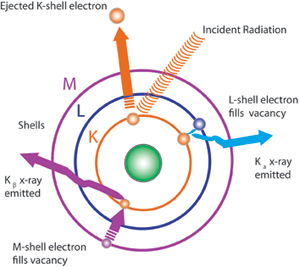In FPXRF analysis, a process known as the photoelectric effect is used in analyzing samples. Fluorescent X-rays are produced by exposing a sample to an X-ray source that has an excitation energy similar to, but greater than, the binding energy of the inner-shell electrons of the elements in the sample. Some of the source X-rays will be scattered, but a portion will be absorbed by the elements in the sample. Because of their higher energy level, they will cause ejection of the inner-shell electrons. The electron vacancies that result will be filled by electrons cascading in from outer electron shells; however, since electrons in outer shells have higher energy states than the inner-shell electrons they are replacing, the outer shell electrons must give off energy as they cascade down. The energy is given off in the form of X-rays, and the phenomenon is referred to as X-ray fluorescence. Because every element has different electron shell energies, each element emits a unique X-ray at a set energy level or wavelength that is characteristic of that element. The elements present in a sample can be identified by observing the energy level of the characteristic emission X-rays. The intensity of the emission X-rays is proportional to the concentration and can be used to perform quantitative analysis.

The K, L, and M shells are those commonly involved in FPXRF analysis. A typical emission pattern, or emission spectrum, for a given element has several peaks generated from the emission of X-rays from those shells. Each of these shells also has alpha and beta emissions at different energies. For example, K alpha spectra for lead are around 74.96 kev, while K beta are found at 84.92 kev. L alpha for lead are around 10.55 and L beta 12.61kev. Note that since XRF affects inner shell and not bonding electrons, the XRF spectrum of an element is independent of its chemical form. See the Table for individual element Kev values for K and L shell electrons.

Top of Page

An XRF analyzer consists of three major components: (1) a source that generates X-rays (a radioisotope or X-ray tube); (2) a detector that converts X-rays emitted from the sample into measurable electronic signals; and (3) a data processing unit that records the emission or fluorescence energy signals and calculates the elemental concentrations in the sample. The following sections describe each of the components in greater detail.

Sources

Detectors

Software

Top of Page

To perform an analysis, a sample is positioned in front of the plastic film measurement window of the probe, and measurement of the sample is initiated, usually by depressing a trigger or start button. Doing so exposes the sample to the X-ray radiation. The length of time the sample is exposed is referred to as the count time. Fluorescent and backscattered X-rays from the sample reenter the analyzer through the window and are counted by the instrument's detector. X-rays emitted by the sample at each energy level are called "counts." The detector records the counts, measures the energy of each X-ray, and builds a spectrum of element peaks on a multichannel analyzer (MCA). The unit's software integrates the peaks to produce a measurement of concentrations of elements and, usually, the standard deviation for each analyte based on the counting statistics. At the completion of the exposure time, the instrument software statistically computes a concentration from the readings collected from each energy level along the spectrum.

Count times from 30 seconds per source to as long as 600 seconds per source can be employed, depending on the data quality needs of the project. As count times increase, the detector collects a larger number of X-rays from the sample, including more X-rays from elements that are present at comparatively lower concentrations. In general, a 4x increase in count time results in a 2x decrease in detection limits, although there will be diminishing returns beyond several hundred seconds. Also, the longer the count time, the greater the reading's precision (but not necessarily accuracy).

In Situ and Intrusive Analysis

An FPXRF detector can be operated in the in situ or the intrusive mode. The particular requirements of the job, such as the required detection limits or data sample precision and accuracy, and the purpose of sampling—for field screening or for quantitative analysis—will determine which mode is appropriate and what count times are needed.

• In Situ

  XRF instrument in situ analysis refers to the rapid screening of soil in place and is generally used to locate hotspots. For in situ operation, the window of the probe is placed in direct contact with the surface to be analyzed and a trigger is pulled. Because analyses in this mode typically are completed very quickly (in less than one minute) and heterogeneity of the samples (both in terms of matrix and element concentration) can be a concern, it is recommended to take three to four measurements in a small area and then average the values to determine the concentrations of target elements. Care should be taken to ensure good contact with the sample (i.e., not on uneven surfaces, rocks, sticks, etc.) to limit x-ray backscatter and measurement variability in this mode.

• Intrusive

  Intrusive analysis is used to ensure greater precision and accuracy when lower detection limits are needed. These goals are achieved through more extensive sample preparation and longer analysis times to reduce heterogeneity among samples and increase the sensitivity of the instrument, respectively. For intrusive operation, a sample is collected, prepared (usually by homogenizing, drying, grinding, and sieving), and placed in a sample cup that has a transparent Mylar® or polyester film window. The sample cup is placed under the probe window (some units provide a safety cover for intrusive analysis) and analyzed. Handheld FPXRF instruments can analyze samples in either mode, while transportable instruments are generally limited to intrusive samples. Preparation of samples is discussed in greater detail in the performance specifications section.

Top of Page

Instruments with X-ray tubes and silicon drift detectors are capable of analyzing sodium through plutonium elements (generally excluding the noble gases) with varying detection limits. Note that low voltage (40-50 kV) X-ray tubes may limit the query to L lines in high Z elements (Barium and higher, Palmer undated 2011) Also, some instruments have the capability to create a vacuum or use a helium purge system to eliminate air in the space in front of the detector, which will lower its detection limits. This ability is very useful for lower-weight elements (e.g., magnesium and aluminum). Note that the software and emission source of a given instrument may be targeted toward a much smaller range of elements.

The radioisotope sources that have been standard in FPXRF units are Fe-55, Cd-109, Am-241, and Cm-244. Elements that those sources are commonly used to analyze include:

Source	Activity (mCi)	Half-Life (Years)	Excitation Energy (keV)	Elemental Analysis Range
Fe-55	20-50	2.7	5.9	Sulfur to Chromium K Lines Molybdenum to Barium L Lines
Cd-109	5-30	1.3	22.1 and 87.9	Calcium to Rhodium K Lines Tantalum to Lead K Lines Barium to Uranium L Lines
Am-241	5-30	432	26.4 and 59.6	Copper to Thulium K Lines Tungsten to Uranium L Lines
Cm-244	60-100	17.8	14.2	Titanium to Selenium K Lines Lanthanum to Lead L Lines

Source: EPA SW-846, Method 6200

Top of Page

Performance specifications include information about interferences, detection limits, calibration, sample preparation, quality control, and precision and accuracy.

Interferences

A variety of factors can affect the detection and quantification of elements in a sample. Some factors can be prevented or minimized through careful preparation and sample design; others are natural effects that must be taken into consideration. To produce useful data, it is important that the analyst understand the relevant interferences.

• Elemental Matrix Effects

  The presence of different elements and their concentrations in a sample can lead to X-ray absorption and enhancement phenomena. For example, iron tends to absorb copper X-rays and will interfere with low levels of chromium, and high levels of lead will interfere with low levels of arsenic. The effects can be corrected mathematically through the FPXRF instrument's software. See the Table for individual element Kev values for K and L shell electrons.

• Physical Matrix Effects

  Matrix effects can cause a great deal of variation in sample analyses. Because XRF is predominantly a surface measurement (X-rays penetrate a few millimeters at most into soil), the physical matrix of the sample is important. Physical matrix effects result from variations in the physical character of the sample soils, such as particle size, uniformity, homogeneity, and condition of the surface. If the data quality objective is to provide an accurate quantitative concentration, every effort should be made to homogenize the soil samples thoroughly before analysis. A discussion of this process is given in the sample preparation section.

• Moisture Effects

  Moisture content above 20 percent may cause problems because moisture alters the soil matrix for which the FPXRF has been calibrated. Moisture can also have a dampening effect on the return signal. These problems can be minimized by drying., preferably in a convection or toaster oven. Drying by microwave is not recommended because it can increase variability between the FPXRF data and confirmatory data and can cause arcing if fragments of metal are present in the sample (EPA SW-846). Also, if a comparison between FPXRF data and confirmatory data is made, ensure to account for results reported on a wet or dry weight basis, especially when comparing to ICP.

Sampling Effects

In environmental samples, typical X-ray penetration depths range from 0.1 millimeter (mm) to 1 mm. Inconsistent positioning of samples in front of the probe window is a potential source of error because the X-ray signal decreases as the distance from the source increases. Maintaining a consistent distance between the window and the sample minimizes that problem. For best results, the window of the probe should be in direct contact with the sample or material housing the sample, such as mylar or poly films over cups, or plastic bag.

Detector Resolution Effects

The resolution of the detector may cause problems in analyzing some elements. If the energy difference between the characteristic X-rays of two elements (as measured in eV) is less than the resolution of the detector in eVs, the detector will not be able to resolve the peaks. In other words, if two peaks are 240 eVs apart, but the resolution of the detector is 270 eV, the detector will have difficulty in differentiating those peaks. A common example is the overlap of the arsenic K_a peak with the lead L_a peak. With the use of mathematical corrections that subtract an estimated L_a lead interference, lead can be measured from the lead L_b peak, and arsenic still can be measured from the arsenic K_a peak. The concentration of arsenic will be less precise, however, because of the statistical estimation of the lead L_a concentration.

Detection Limits

An FPXRF operator must consider two types of detection limits: instrument detection limits (DL) and method detection limits (MDL). A DL is the absolute threshold concentration of a given element that a particular instrument can resolve, as determined by the standard deviation (SD) of an individual analytical result. Instruments equipped with SDDs can achieve DLs of <5 to <50 ppm for most elements between potassium and plutonium (e.g., <5 ppm for zinc, lead, and mercury and <10 ppm for chromium, copper, and cadmium).

MDLs depend on the analytical method (such as preparation and analysis times) and sample matrix and may be higher than DLs. The results of replicate measurements of a low-concentration sample can be used to generate an average site-specific MDL. The MDL is defined as three times the SD of the results for a replicate analysis of a low-concentration sample. XRF users should be aware that many instrument configurations will report a measured value (as a function of counting statistics) that is less than 3 SDs of the counting statistics as a non-detect. In some instances it may be of value to use a "detected" number even if it is less than 3 SDs (e.g., statistical evaluations of the data). In these instances it may be worth while to talk with the manufacturer about whether these numbers can be made available.

Top of Page

FPXRF units are calibrated by any of several methods. The methods will vary according to the make of the unit and the intended use of the data, such as for screening or for quantitative analysis.

• Fundamental Parameters Calibration

  The fundamental parameters (FP) calibration is a "standardless" calibration. Rather than calibrating a unit's calibration curve by measuring its response to standards that contain analytes of known concentrations, FP calibration relies on the known physics of the spectrometer's response to pure elements to set the calibration. Built-in mathematical algorithms are used to adjust the calibration for analysis of soil samples and to compensate for the effects of the soil matrix. The FP calibration is performed by the manufacturer, but the analyst can adjust the calibration curves (slope and y-intercept) on the bases of results of analyses of check samples, such as standard reference materials (SRM), which are analyzed in the field. This mode is best for samples containing elements that can be detected by XRF (i.e., alloys, well characterized samples, and samples containing relatively high concentrations of elements) (Palmer 2011).

• Empirical Calibration

  In performing an empirical calibration, a number of actual samples, such as site-specific calibration standards (SSCS), are used, and the instrument's measurements of the concentrations of known analytes in the samples are taken. Empirical calibration is effective because the samples used closely match the sample matrix. SSCSs are well-prepared samples collected from the site of interest in which the concentrations of analytes have been determined by a reference method, such as inductively coupled plasma, atomic absorption, or other methods approved by the regulatory agency. The standards should contain all the analytes of interest as well as interfering analytes. Manufacturers recommend the use of 10 to 20 calibration samples to generate a calibration curve. When comparing the methods for calibration, take note of the acid digestion-spike recoveries (efficiency) of the analytical method to assure that the lab method data is compatible with the XRF data. Poor efficiency means that a direct comparison of the data will be difficult. Total digestion (e.g. SW 846 Method 3052) can be expensive and may not be the best analytical value if a 1:1 calibration is insisted upon. One solution is using a reference method along with the XRF method in a collaborative fashion. For a discussion of laboratory versus field determined values see Section 2.7 of ITRC 2003.

• Compton Normalization

  The Compton normalization method incorporates elements of both empirical and FP calibration. A single well-characterized standard, such as an SRM or SSCS, is analyzed, and the data are normalized for the Compton peak. The Compton peak is produced from incoherent backscattering of X-ray radiation from the excitation source and is present in the spectrum of every sample. The intensity of the Compton peak changes as various matrices affect the way in which source radiation is scattered. For that reason, normalizing to the Compton peak can reduce problems with matrix effects that vary among samples. Compton normalization is similar to the use of internal standards in analysis for organic analytes.

• Sample Preparation

  Procedures for sample preparation for in situ and intrusive analysis vary considerably because the two methods serve completely different purposes. Sample preparation for in situ analysis is fairly straightforward, while sample preparation for intrusive analysis can be fairly complicated, depending on the data quality required.

  In situ or "point-and-shoot" analysis requires little sample preparation and is generally used for field screening of hotspots:

  • First, any unrepresentative debris (e.g., rocks, pebbles, leaves, vegetation, roots) should be removed from the surface of the soil.
  • Second, the surface must be smooth to allow the probe window to make good contact with the soil surface.
  • Finally, the surface of the soil should not be saturated to the point that ponded water is present.

  For an "in situ prepared" sample, which provides for better quantitation and detection limits:

  • Soil from the sampling point is collected, and all unrepresentative debris (e.g., rocks, pebbles, leaves, vegetation, roots) is removed.
  • The soil is placed in a plastic bag and thoroughly homogenized. At a minimum, this should include mixing and breaking of aggregate material to best obtain a uniform particle size.
  • The sample probe is placed directly on the bag for analysis. In very rare cases, plastic bags can have potential interference (often attributable to bag construction [ribbed, overly thick, or crinkled tend to increase x ray scatter and variability] and moisture within the bag). This potential for interference should be checked by taking repeated measurements of NIST standards and/or well characterized site samples with and without shooting through the bags.
  • When performing the analysis, a series of measurements is recommended to understand sample heterogeneity and to generate an average concentration. For example, one could use two or more measurements on the front side of the bag followed by two or more on the back side of the bag.

  For intrusive analysis, the sample first must be collected and then prepared for analysis in a sample cup or bag. Some or all of the following steps may be necessary, depending on the data quality needed:

  • Any large, unrepresentative debris should be removed from the sample.
  • The most important preparation step is thorough homogenization. Mixing the sample in a plastic bag and breaking any aggregate material to best obtain a uniform particle size works well. If a high degree of precision and accuracy is not required, the sample can be analyzed in the bag. A representative bag should be tested to determine if it contains any trace elements of concern and if it interferes with emission or return X-rays. Testing can be done by taking repeated measurements of NIST standards and/or well characterized site samples with and without shooting through the bags.
  • If the sample contains more than 20 percent moisture, the sample should be dried, preferably in a convection or resistive oven. Drying in a microwave oven is discouraged because doing so can increase the variability between the FPXRF data and confirmatory data, and arcing can occur when metal fragments are present in the sample. Note that mercury is volatile, and if it is a suspected contaminant of concern, the samples should be air dried.
  • If a high degree of precision and accuracy is required or if a particular soil fraction is of interest (e.g., fines <60 mesh to evaluate dust inhalation), the sample should be passed through a sieve. If the sample is not wet (has a moisture content of less than 20 percent) and is not high in clay content, the sample can be sieved in the field before it is placed in a container; otherwise, the sample is ground with a mortar and pestle or ball mill and passed through a 40- or 60-mesh sieve after drying.
  • Finally, the sample is placed in a 31- or 40-mm polyethylene cup and covered with Mylar film.
• Quality Control

  Ensuring that the data generated by FPXRF analysis are of a known quality is vital to ensuring the usefulness of those data, regardless of their purpose. Quality control (QC) measures take several forms and can be performed in the field, during sample analysis, and after sample data have been collected. The amount and type of QC necessary will depend on the project's data quality objectives. A higher degree of QC is necessary to produce defensible, definitive data, but analytical results from intrusive analysis have been demonstrated to compare favorably with results obtained through traditional laboratory methods, given that sample preparation has been thorough and QC adequate. By nature, results obtained in situ are of lower quality because of the lack of sample preparation. A typical QC program might include the following measures:

  • An energy calibration check sample.
  • An instrument blank.
  • A method blank.
  • A calibration verification check sample, which is usually accomplished through a series of NIST standards like 2709b, 2710b, and 2711b.
  • A precision sample.
  • A confirmatory sample (Note: Be sure to specify that the analysis is for total metals, not extractable.).

Top of Page

XRF costs vary significantly ($25,000 to $50,000). Instrument design and accessories affect instrument prices. Manufacturers should be contacted directly for cost information. Also, instruments can be rented, and some consulting firms offer FPXRF surveys as a service.

Top of Page